In this article, I will explain 14 practical uses of the new GROUPBY function in Microsoft Excel. This function overlaps with some of the uses of a pivot table. However, there are some differences between the two approaches which make both still useful depending on your requirements.
To illustrate the use of GROUPBY function, I will use the following dataset. It is a list of all 582 Test Matches played by Indian Cricket team until recently.
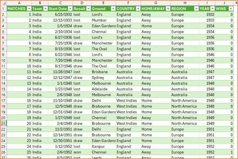
Here are the definitions of important columns.
- MATCHES: Represents the sequence of matches played. Uniquely identifies each match.
- Result: Result of the match. “won” indicates that India won the match
- COUNTRY: Opposition team
- HOME/AWAY: Whether the match was played in home (India) or away (other countries)
- REGION: Region where the opposition country belongs to
- YEAR: Year when the match was played
- WINS: 1 if India won; 0 otherwise.
I name this table T_RESULTS. Converting your dataset to a table is very helpful and is recommended.
Video Tutorial
The syntax for the GROUPBY function is below:
GROUPBY(row_fields,
        values,
        function,
        [field_headers],[total_depth],[sort_order],[filter_array],[field_relationship])
Microsoft’s Help article
Now, let’s get started with our formulas using the GROUP BY function.
1. Simple Aggregation of a Value column by an attribute
=GROUPBY(T_RESULTS[[#All],[COUNTRY]],
         T_RESULTS[[#All],[WINS]],
        SUM)
This is the most basic use of the GROUPBY. We use only the required parameters for this function.
The above formula groups by data by COUNTRY column and sums up the WINS column.
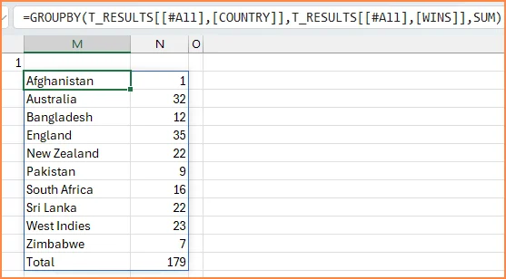
The result is the number of wins against each country. Please note that the total appears at the bottom by default.
We used the SUM function for aggregating in this example. You can also use others like MIN, MAX, AVERAGE, PRODUCT and more.
2. Formatting – Adding Header
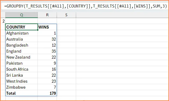
One obvious thing to note in the above result is that there is no header in the output. To change that, we update formula as shown below.
=GROUPBY(T_RESULTS[[#All],[COUNTRY]],
         T_RESULTS[[#All],[WINS]],
         SUM,
         3)
We add an optional 4th parameter in the formula. Choosing 3 displays the header
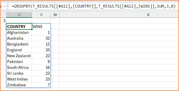
3. Formatting – Totals
We have control over display of totals. If we don’t want to display the total or if we want to display the total on the top (instead of bottom), we can choose parameters accordingly.
=GROUPBY(T_RESULTS[[#All],[COUNTRY]],
         T_RESULTS[[#All],[WINS]],
         SUM,
         3,0)
As an optional 5th parameter, choosing 0 will remove totals. 1: Grand Total; 2 Grand total and Subtotals; -1: Grand Total at the top; -2: Grand and Subtotals at top.
4. Formatting – Sorting
By default, the data is sorted alphabetically by country. We have control over sorting order and sorting column. We can enter the 6th parameter in the formula to control sorting.
=GROUPBY(T_RESULTS[[#All],[COUNTRY]],
         T_RESULTS[[#All],[WINS]],
         SUM,
         3,0,-2)
Entering 2 tells Excel to sort by the second column in output, which is the WINS column. Negative 2 tells Excel to sort descending.
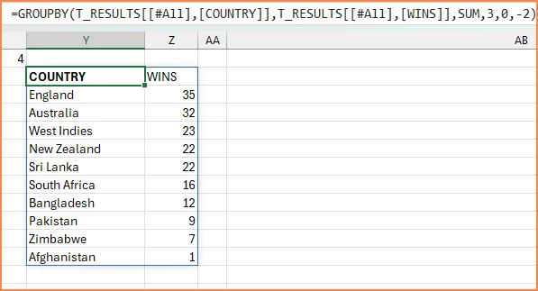
The result is a table of wins against each country, sorted in descending order by Wins.
5. Filtering with GROUPBY
So far, we have used GROUPBY to summarize data from the entire dataset. We can also apply conditions or filters to remove/include specific rows of data. This is done using the optional 7th parameter.
Let’s say we want to show the wins against each country, but only from matches played in India (Home). We can add the following condition in the 7th parameter: T_RESULTS[[#All],[HOME/AWAY]]=”Home”
=GROUPBY(T_RESULTS[[#All],[COUNTRY]],
         T_RESULTS[[#All],[WINS]],
         SUM,
         3,1,2,
         T_RESULTS[[#All],[HOME/AWAY]]="Home")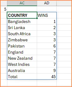
6. Multiple aggregations on a value column – horizontal layout
Until now, we have seen only a single aggregation function applied. We can also do multiple aggregations on a single value column.
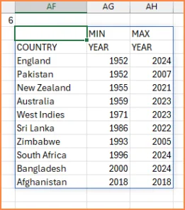
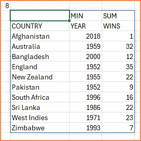
Let’s say we want to find the earliest year of victory and latest year of victory against each country.
=GROUPBY(T_RESULTS[[#All],[COUNTRY]],
         T_RESULTS[[#All],[YEAR]],
         HSTACK(MIN,MAX),
         3,0,2,
         T_RESULTS[[#All],[Result]]="won")
In the above formula, we use HSTACK (MIN, MAX) to let Excel use two aggregations on the YEAR column. The result is as shown below.
7. Multiple aggregations on a value column – vertical layout
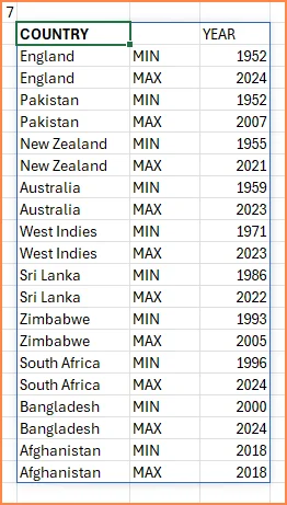
In some occasions, we may want the aggregation results to be displayed vertically.
=GROUPBY(T_RESULTS[[#All],[COUNTRY]],
         T_RESULTS[[#All],[YEAR]],
         VSTACK(MIN,MAX),
         3,0,2,
         T_RESULTS[[#All],[Result]]="won")
We can use the VSTACK instead of HSTACK.
8. Aggregations on multiple value columns (adjacent)
Let’s say we want to show the earliest year of victory along with the total number of wins. We need to apply aggregations to two different value columns (YEAR and WINS). that are placed next to each other in our table.
=GROUPBY(T_RESULTS[[#All],[COUNTRY]],
         T_RESULTS[[#All],[YEAR]:[WINS]],
         HSTACK(MIN, SUM),
         3,0,1,
         T_RESULTS[[#All],[Result]]="won")
In the formula, T_RESULTS[[#All],[YEAR]:[WINS]] represents the columns starting from YEAR until WINS. When we apply HSTACK(MIN, SUM) aggregations, MIN applies to the YEAR column and SUM applies to the WINS column.
9. Aggregations on multiple value columns (non-adjacent)
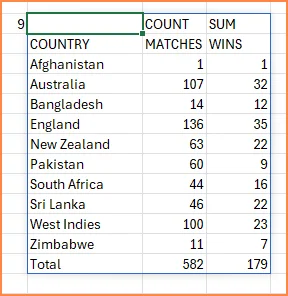
if the value columns are not next to each other, we can still handle it. For example, we want to show the number of matches played and number of wins. These two value columns (MATCHES, WINS) are not next to each other in our source table.
=GROUPBY(T_RESULTS[[#All],[COUNTRY]],
         HSTACK(T_RESULTS[[#All],[MATCHES]],T_RESULTS[[#All],[WINS]]),
         HSTACK(COUNT, SUM),
         3,1,1)
In this formula, we apply HSTACK to the two columns MATCHES and WINS. We also apply HSTACK as before to do multiple aggregations (COUNT, SUM).
10. Aggregations by multiple row fields (hierarchy)
We can also have multiple row fields when we summarize/group by. For example, if we want to show the number of wins grouped by Region and Country.
=GROUPBY(HSTACK(T_RESULTS[[#All],[REGION]],T_RESULTS[[#All],[COUNTRY]]),
         T_RESULTS[[#All],[WINS]],
         SUM,
         3,2,-3)
Similar to how we used HSTACK in earlier examples, we can HSTACK Region and Country columns.
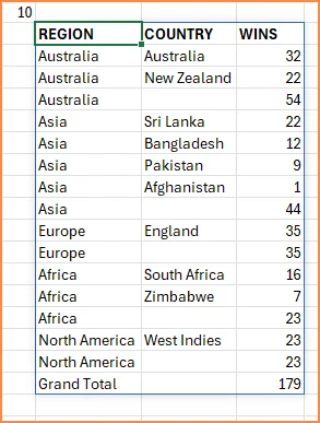
One thing to note here is that we have enabled subtotals in the above formula. 5th parameter is set to 2, which enables grand and subtotals. In this scenario, the sorting is done descending based on WINS column (our 6th parameter is -3). However, the hierarchy applies by default. This means the REGION with highest wins is at the top and region with second highest wins will go next. It is not the wins by country and it’s wins by region that takes priority in sorting. That’s why England with 35 is lower in the list behind Asian countries, since Asia as a region has 44 wins and Europe only 35. Asia goes above Europe.
11. Aggregations by multiple row fields (Table)
If we want to sort by value column only then we have to choose the 8th parameter available in the function.
=GROUPBY(HSTACK(T_RESULTS[[#All],[REGION]],T_RESULTS[[#All],[COUNTRY]]),
         T_RESULTS[[#All],[WINS]],
         SUM,
         3,0,-3,
         ,
         1)
I have entered 1 as the 8th parameter in the above formula. This setting allows sorting ignoring any hierarchy in our data.
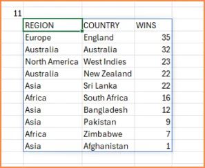
In this result, the Countries are sorted based on Wins
It is important to note that when we choose this setting, the subtotals cannot be enabled.
12. ArraytoText
A special case of aggregation is ARRAYTOTEXT. Here, we can combine multiple values in a single column and display the array as concatenated text. For example, I want to see the results of matches played after 2021 by country.
=GROUPBY(T_RESULTS[[#All],[COUNTRY]],
         T_RESULTS[[#All],[Result]],
         ARRAYTOTEXT,
         3,0,,
         T_RESULTS[[#All],[YEAR]]>2021)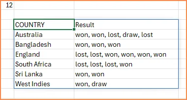
The result is a table where the recent match results for each country are shown.
13. Refer to GROUPBY result in another formula
When we develop reports in Excel, we can also use GROUPBY to create an intermediate dataset which is used in another formula downstream. If we have entered a formula using GROUPBY function in cell A3, we can now refer to that result by simply adding a #.
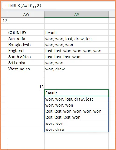
=INDEX(AW3#,,2)In the simple formula, we are extracting only the second column of the GROUPBY result in cell AW3.
14. Conditional formatting on GROUPBY results
To make the results of a GROUPBY easier to read when we have subtotals, we can use the following approach.
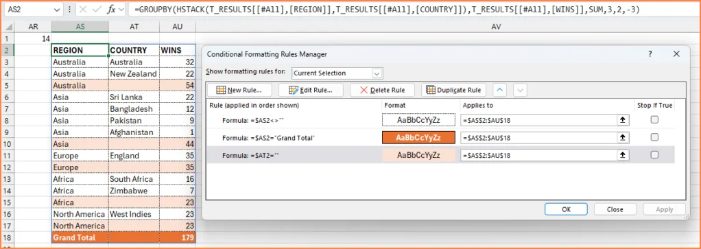
The first rule creates the border around all the cells.
The second rule creates a dark orange fill with white bold font for the Grand Total row.
The third rule creates a light orange fill for subtotal rows.


