How to Unpivot Data in Excel using formulas?

Unpivoting data is a common task in data transformation. In this article, we will learn how to use simple formulas to unpivot. It can also be done using Power Query. Both approaches have their pros and cons. Unpivoting using formulas is a good technique to have in your arsenal.

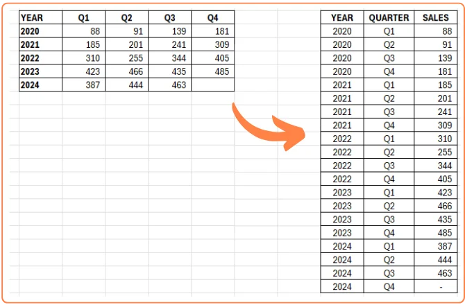
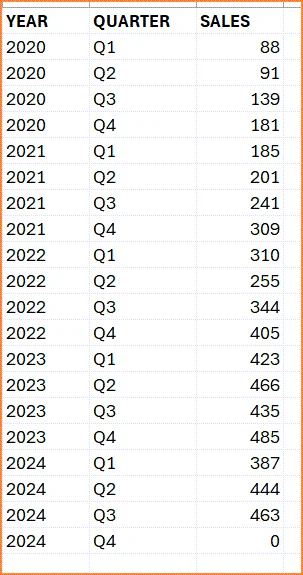
Using the data on the left, we will be writing 3 formulas to create the YEAR, QUARTER and SALES columns on the right.

Setup

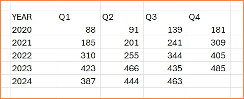
The data we will use for this exercise is Tesla car sales (in thousands) data by quarter.

Video Tutorial

Step 1 : Convert the data to a table

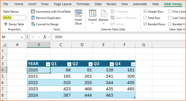
Convert the data to a table by selecting all the cells (with data) and pressing Ctrl+T.

Name the table DATA.

Step 2: Create the YEAR column

Step 2.1 Generate a sequence of 1s

The data is for 5 years and 4 quarters. Each year should be repeated 4 times. Hence we enter this formula.

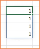
= SEQUENCE(4,,1,0)

The formula generates a sequence of 4 1s as shown below.

Step 2.2 Repeat the Years 4 times

Update the formula

=CHOOSECOLS(DATA[YEAR],SEQUENCE(4,,1,0))

The result is

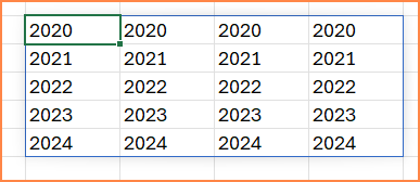
The 5 years are repeated 4 times in 4 columns.

Step 2.3 Convert the data to a single column

To convert to a single column of values, we can use the TOCOL function. Update the formula as

=TOCOL(CHOOSECOLS(DATA[YEAR],SEQUENCE(4,,1,0)))

Step 3: Create the QUARTER Column

The formula is similar in concept to the formula we used for the YEAR column. But there are some differences which we will explain.

Step 3.1 Create the sequence of 1s

We need to create each quarter (example Q1) five times, since we have 5 years in data. So, we use 5 as our parameter in the SEQUENCE function.

= SEQUENCE(5,,1,0)

Generates a sequence of 5 1s.

Step 3.2 Repeat the Quarters 5 times.

Update the formula to this

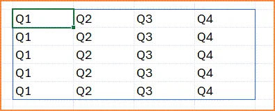
=CHOOSEROWS(DATA[[#Headers],[Q1]:[Q4]],SEQUENCE(5,,1,0))

Here, we choose the headers for the 4 quarters, and then pass the result of the sequence function.

This generates the quarters 5 times in 5 rows.

Step 3.3 Convert to a single column

Finally, update the formula to

=TOCOL(CHOOSEROWS(DATA[[#Headers],[Q1]:[Q4]],SEQUENCE(5,,1,0)))

Step 4: Create the SALES column

Creating the sales column is quite straightforward. This simple formula takes all the data in columns Q1, Q2, Q3 and Q4, and then converts to a single column of values.

=TOCOL(DATA[[Q1]:[Q4]])

The result is as shown below.

Notes:

1. We used Quarterly data in this exercise. We can use a similar concept to unpivot monthly, annual or weekly data. The parameter we use in the SEQUENCE function will change: 4 for quarters, 12 for months and 52 or 53 for weeks.
2.  We used 5 years of data in this exercise. You can apply the concept to more or fewer years, by modifying the parameter in the SEQUENCE function.
3. We can make the formulas more dynamic by not hardcoding the parameters to the SEQUENCE function. We can instead count the number of rows and columns using formulas and use them inside the SEQUENCE function.
4. The concept can be applied even to datasets which are not date related. Instead of quarterly data across 5 years, it could be quarterly sales data for each of the 10 products a company produces.
5. If there is missing data in the dataset, we can handle those with minor changes to the formula.