Mastering Excel’s XLOOKUP Function:
Excel’s XLOOKUP function is a game-changer for anyone working with data. Its versatility and power make it an essential tool for simplifying the process of searching and retrieving information within spreadsheets. Whether you’re a beginner or an experienced Excel user, XLOOKUP can transform the way you handle data.
What Makes XLOOKUP Special?
As Excel’s latest lookup function, XLOOKUP is designed to replace and improve upon its predecessors, VLOOKUP and HLOOKUP, by overcoming many of their limitations. With XLOOKUP, you can search for values in a range or array and retrieve corresponding data seamlessly, regardless of whether the search is horizontal or vertical.
In this blog, we’ll explore nine practical examples that demonstrate the incredible flexibility of XLOOKUP, showing you how to maximize its potential for solving real-world challenges.
I have used a list of Employee data to explain the nine cases of using the XLOOKUP function.
Case 1 : Simple lookup of exact match of value
Objective: Finding an Employee’s Salary
In this case we have the List of employees and their salaries.
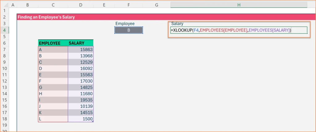
Now to find the salary of “Employee B” use the following XLOOKUP Function
=XLOOKUP(F4,EMPLOYEES[EMPLOYEE],EMPLOYEES[SALARY])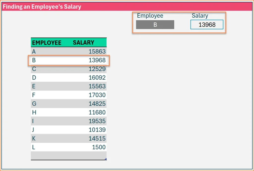
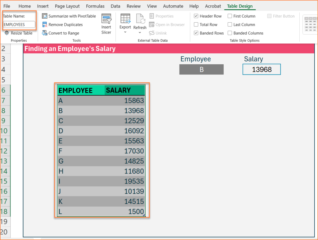
As you can see in the formula the references are meaningful. This is because I have used the Table format to structure the raw data.
To do this, Select the cells of the raw data and click Ctrl + T. And then you can name the table.
When a new employee is added to the table, “XLOOKUP” returns the salary of Employee L.
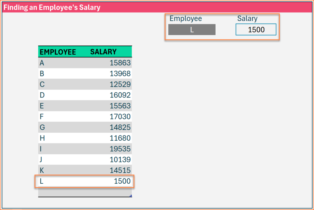
The Table structure makes the formula readable & scalable.
Case 2 : Fill values when there is no match in lookup
Objective: Returning Bonus as “0” for employees not available in the List
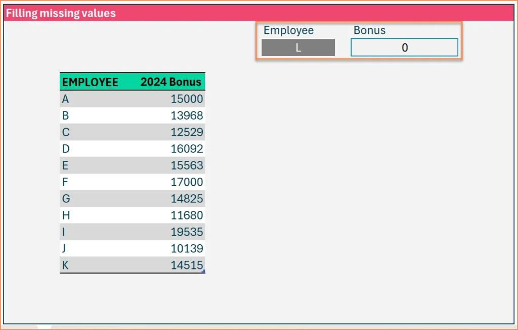
In this case, there’s an employee L who is not in the list of employees who will be receiving a bonus.
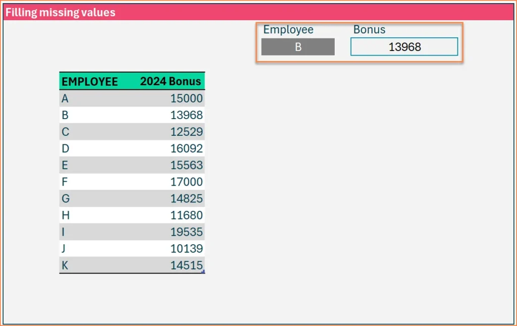
=XLOOKUP(F4,EMPLOYEES2[EMPLOYEE],EMPLOYEES2[2024 Bonus],0)Here, “IF NOT FOUND“ argument is used in the XLOOKUP function. This argument would return the value “0” if no match is found.
When employee L is searched for, the XLOOKUP returns the value “0” as the employee is not available in the list.
Whereas when employee B is searched for it returns the bonus of the employee from the table.
Case 3 : Extract the first or last occurrence
Objective: Finding an Employee’s First or Last Salary
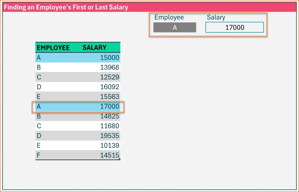
In this case we have multiple records for each employee. An employee has a new record when salary changes.
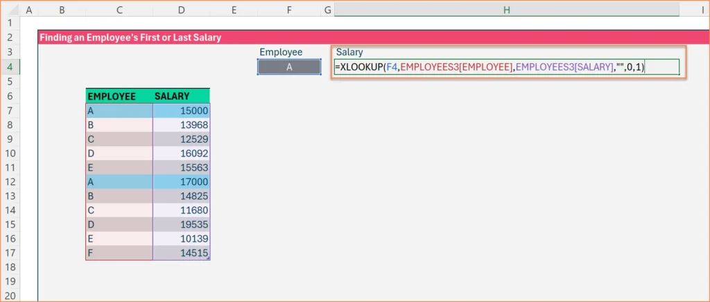
Here we use the sixth argument “Search Mode” in the XLookup function.The fifth argument “Exact Match” is by default set to 0.
In this formula, “Search Mode = 1” will pick the employee that is first from the start. “Search More = -1” will pick the employee that is first from the last.
=XLOOKUP(F4,EMPLOYEES3[EMPLOYEE],EMPLOYEES3[SALARY],"",0,1)First: Now for Employee A, if I use “Search Mode = 1” then the first occurrence of A is returned by excel.
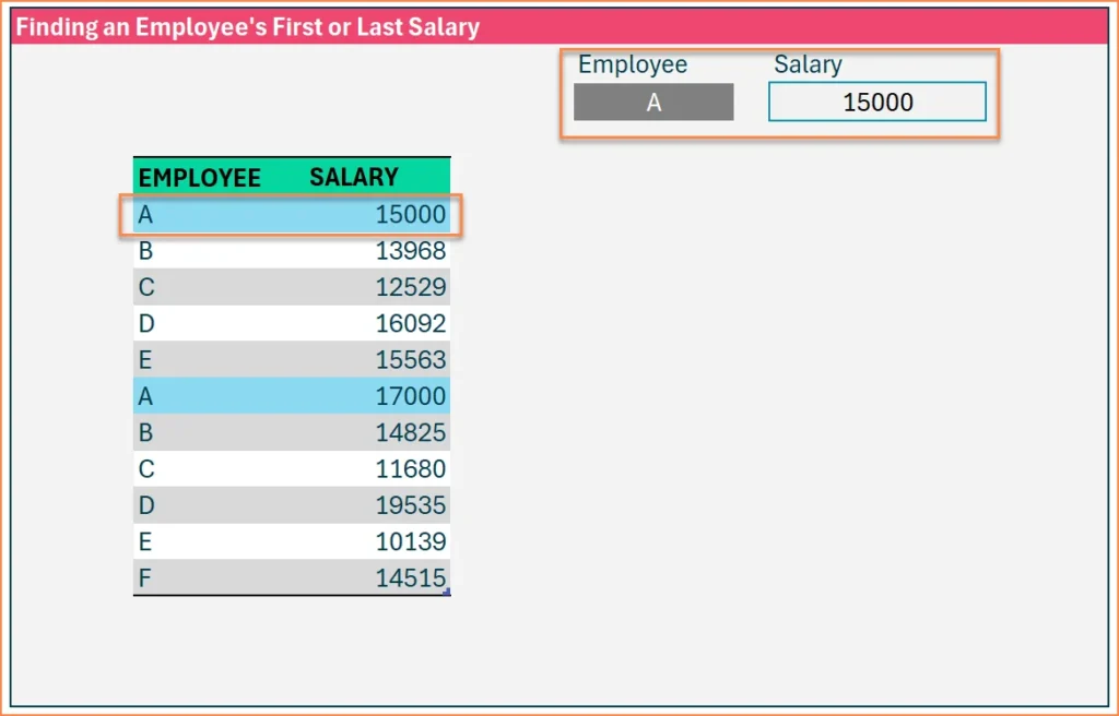
Last: Now, for Employee A, if I use “Search Mode = – 1” then the last occurrence of A is considered by Excel.
Case 4 : Extract lookup values for a range
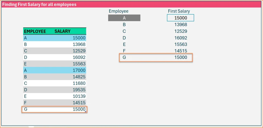
Objective: Finding First Salary for all employees
We have the List of employees and their salaries.
We already know how to get the first salary for the first employee.
=XLOOKUP(F4,EMPLOYEES4[EMPLOYEE],EMPLOYEES4[SALARY],,,1)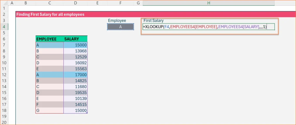
We can find the first salary for all the employees in 3 methods.
Method 1: Click H4 and drag the formula to the cells below.
Method 2: To change the reference F4 to F4:F9 in the formula where F4 to F9 has the list of employee names.
=XLOOKUP(F4:F9,EMPLOYEES4[EMPLOYEE],EMPLOYEES4[SALARY],,,1)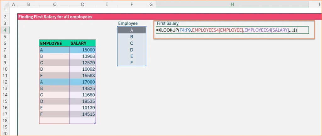
Method 3: If the list of employees is a dynamic array, then we can change F4 to F4# and this will give the array of results. To create a dynamic array of employee names, we can use UNIQUE function.
=XLOOKUP(F4#,EMPLOYEES4[EMPLOYEE],EMPLOYEES4[SALARY],,,1)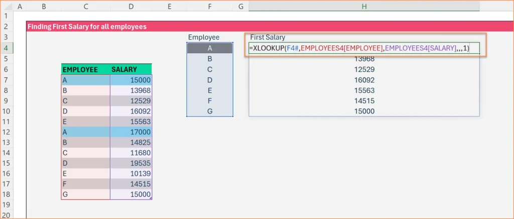
If a new employee is added to the dataset the result will automatically expand to accommodate the new input.
Case 5 : Lookup values when there is no exact match
Objective: Finding rating from another table
Here, we have the List of employees and the performance score.
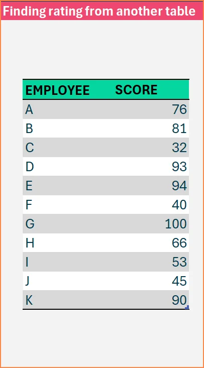
To get the employee’s corresponding score, we use this formula, which fetches the score from column D and returns it in G5.
=XLOOKUP(G4,EMPLOYEES5[EMPLOYEE],EMPLOYEES5[SCORE],"",0,1)
We have a reference table that has the score and its respective rating
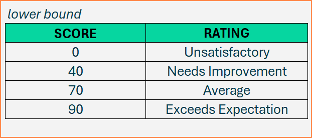
In the lower bound reference table we have the scores 0, 40, 70 and 90 and their respective ratings are Unsatisfactory, Needs Improvement, Average and Exceeds expectation
Now, for Employee F, to get the rating for a score of 40, we use this formula where it looks at the score in cell G5 and returns the rating.
=XLOOKUP(G5,F13:F16,G13:G16,"",-1)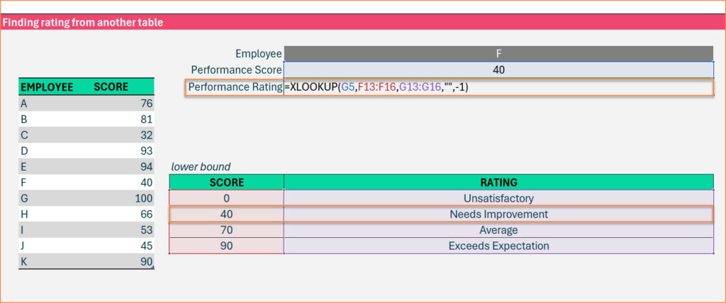
For employee F, the score is 40 and so the performance rating would be “Needs Improvement”
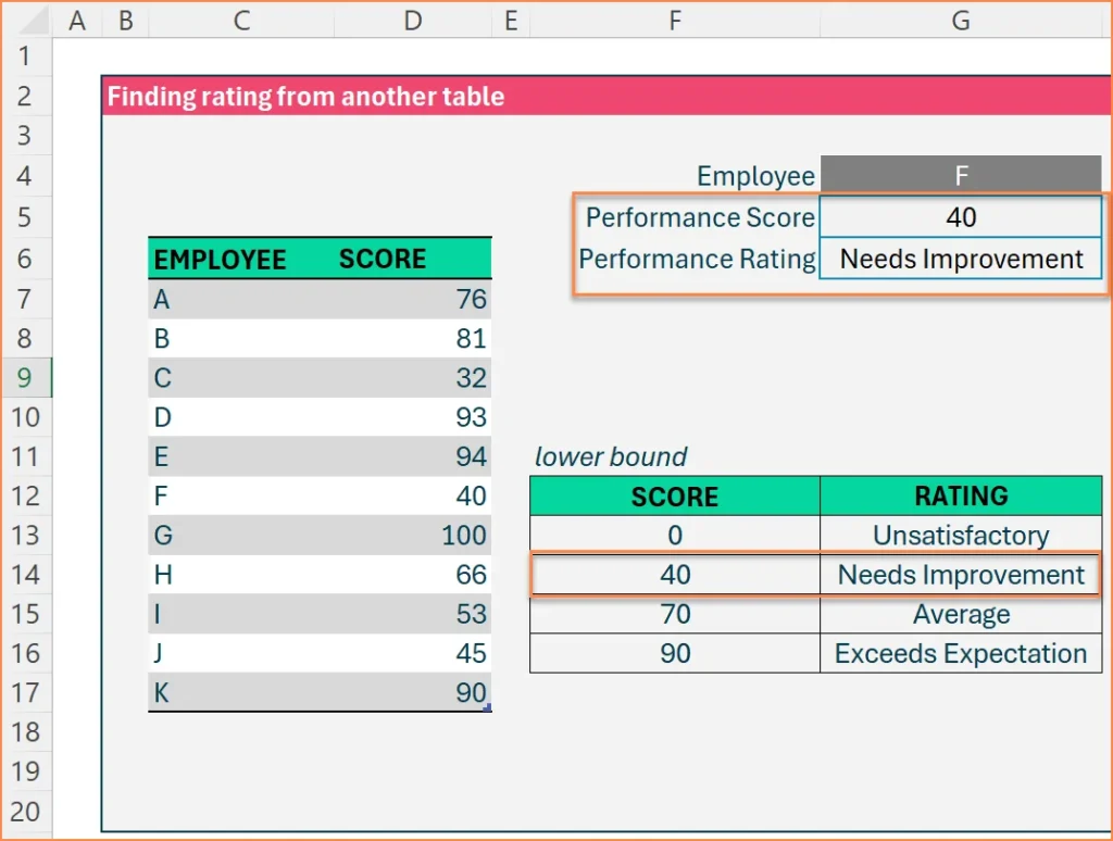
When the value is not an exact match, it will still work since we use match mode equals -1 to get the next lower item.
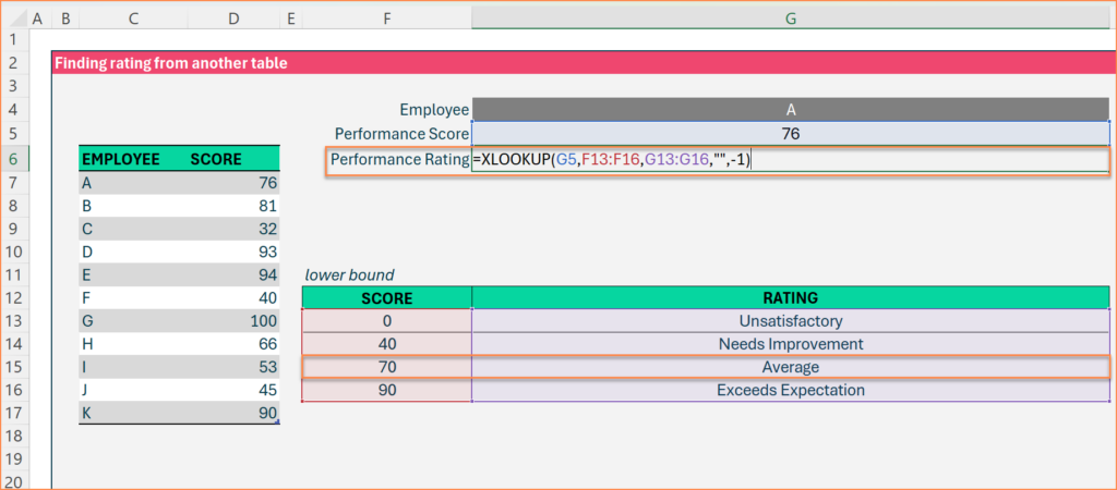
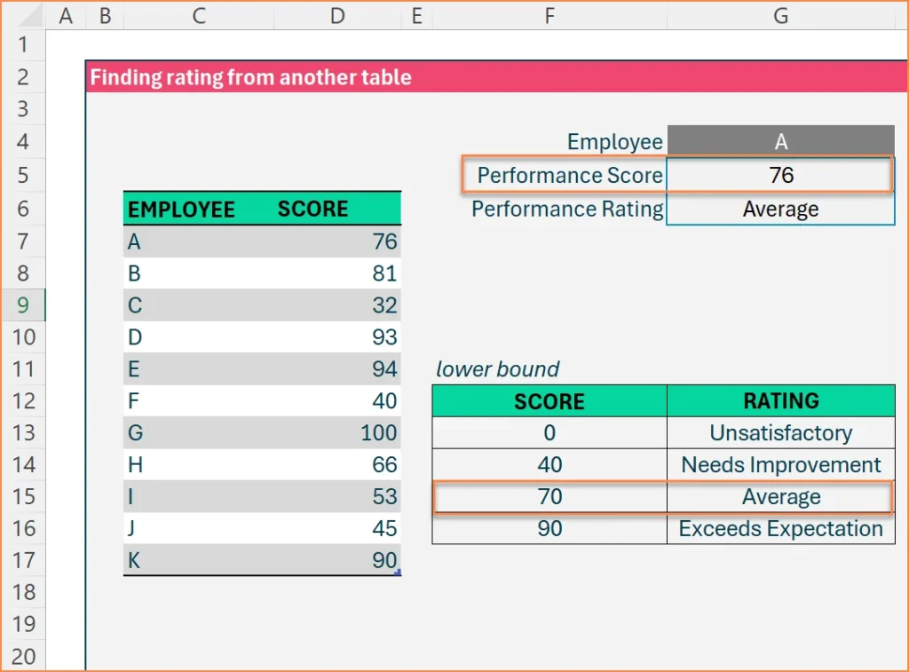
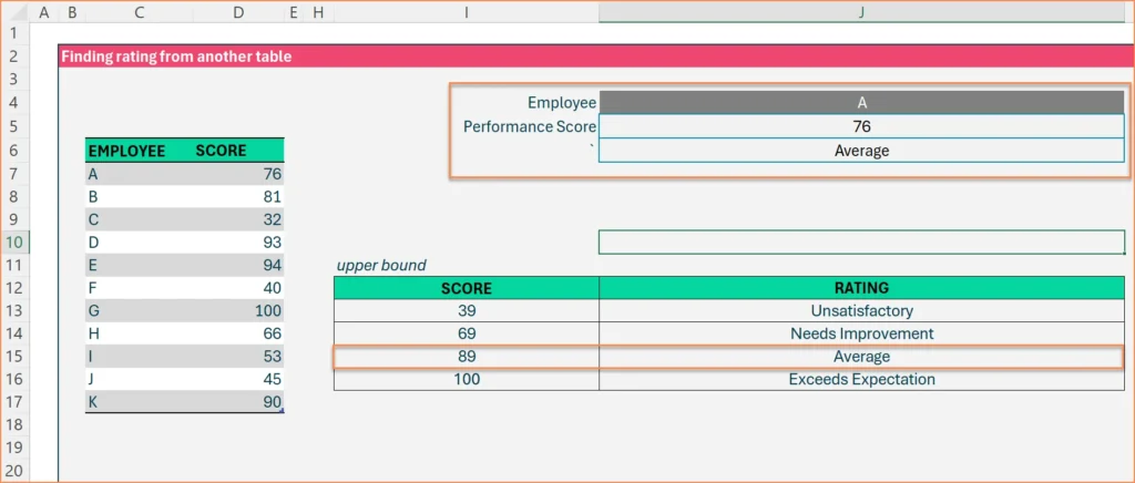
For example, employee A has a score of 76. In this case the next lower item in the reference table is 70 thereby the performance rating will be “Average”.
If your reference table is based on upper bound, we can modify the formula slightly to handle it. The match mode parameter can be set to 1.
=XLOOKUP(G5,I13:I16,J13:J16,"", 1)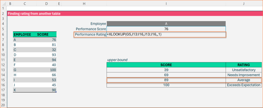
In the upper bound reference table, we have the scores 39, 69, 89 and 100 and their respective ratings are Unsatisfactory, Needs Improvement, Average and Exceeds expectation.
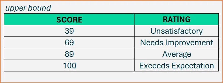
In this case we use match mode equals 1 to get the next larger item. For example, employee A has a score of 76. In this case the next larger item in the reference table is 89 thereby the performance rating will be “Average”.
Case 6 : Lookup with partial match using wildcard
Objective: Finding employees with partial name match
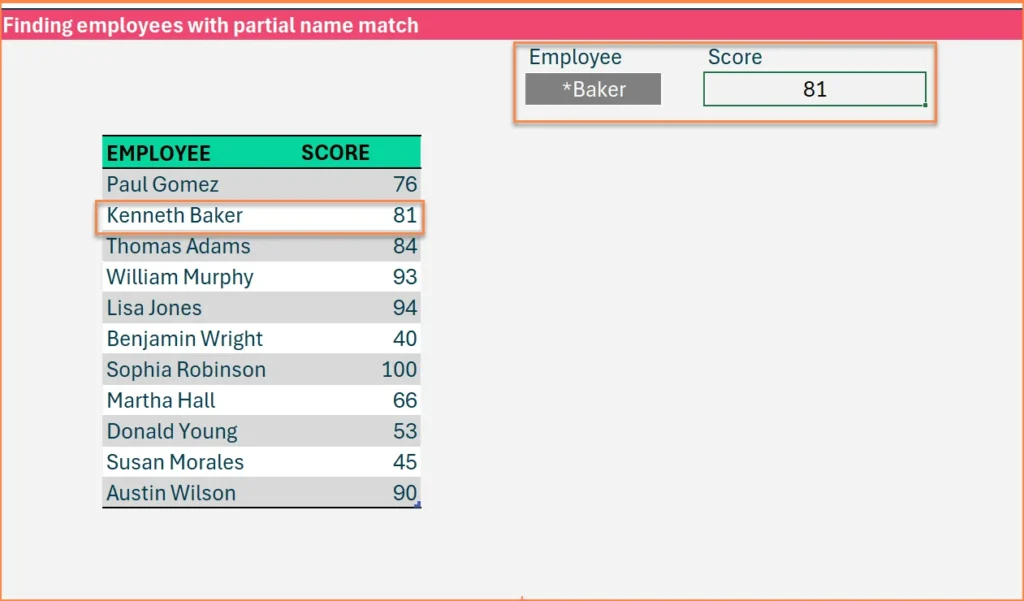
Partial match is used to find the data if a part of the data is already known. Consider we know the first name of the employee and the last name is unknown.
= XLOOKUP(F4,EMPLOYEES6[EMPLOYEE],EMPLOYEES6[SCORE],"",2)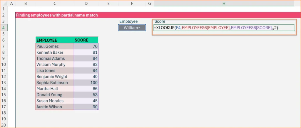
Here “2” represents the” Wild card character” match mode.
Asterisk is used as the wildcard character and this will populate the score for the name that starts with the name ”William”
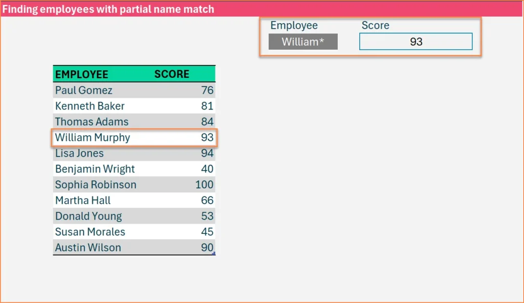
The same can be applied for the name for which the last name is known and the first name is unknown.Here we replace the First name with wild card character “asterisk”. This will populate the score for the name that ends with the name ”Baker”
Case 7 : Retrieve multiple columns when using lookup
Objective: Return multiple columns
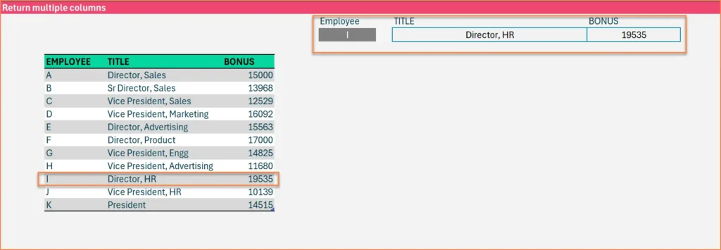
Let’s assume you want to get two pieces of information from the table.
We want to return back both Title and Bonus in the XLOOKUP formula.
=XLOOKUP(G4,EMPLOYEES7[EMPLOYEE],EMPLOYEES7[[TITLE]:[BONUS]])
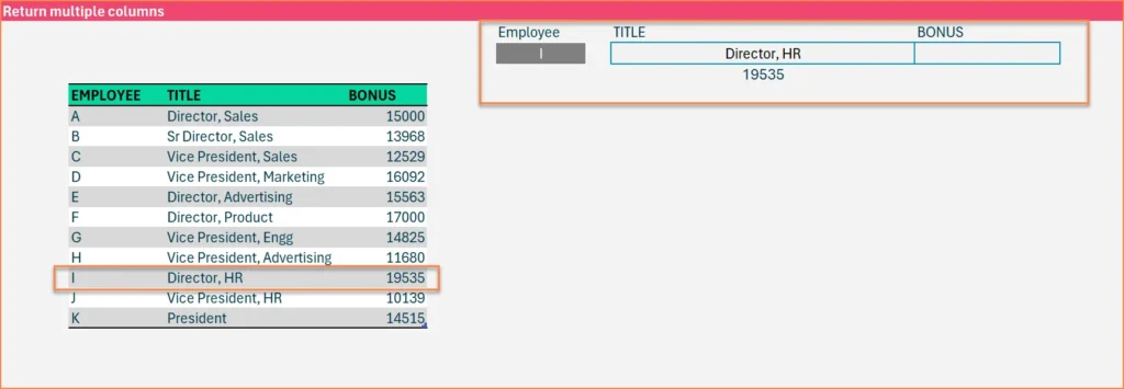
If you want to align both Title and bonus vertically instead of horizontally, then use TRANSPOSE function.
=TRANSPOSE(XLOOKUP(G4,EMPLOYEES7[EMPLOYEE],EMPLOYEES7[[TITLE]:[BONUS]]))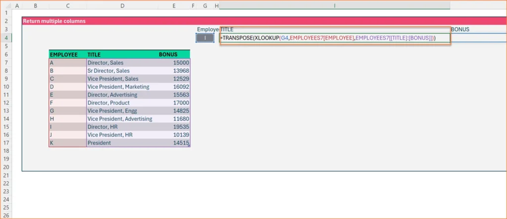
Case 8 : Use multiple conditions when doing Lookup
Objective: Finding employees with name and department match
In this example we will find the score based on two conditions – the Employee name and Department.
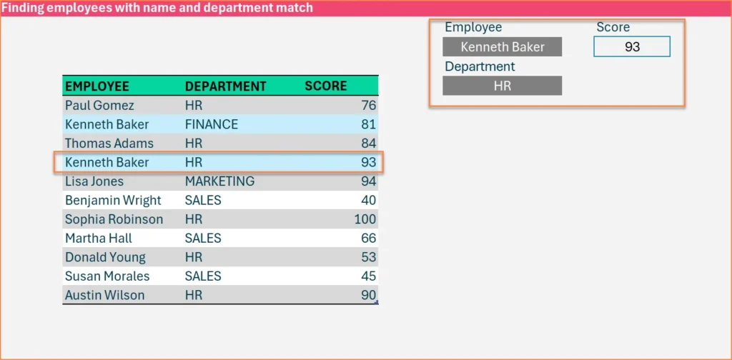
Let’s take the Employee name “Kenneth Baker”. There are two Kenneth Baker, one from the Finance department and another from the HR department.
We are going to use the formula, where the Name matches the name that we are looking for AND the Department matches the same department that we are looking for.
=XLOOKUP(1,(EMPLOYEES8[EMPLOYEE]=G4)*(EMPLOYEES8[DEPARTMENT]=G6),EMPLOYEES8[SCORE],"")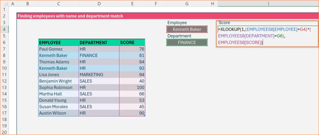
Case 9 : Find the value for the latest record based on date column
Objective: Finding salary based on date
In this example the salary changes over time. However the data is not sorted by date.
We are going to do this in two parts
- Here we use the “MAXIFS” function to get the max date when the employee column matches the employee we are looking for.
max date =MAXIFS(EMPLOYEES9[DATE],EMPLOYEES9[EMPLOYEE],G4)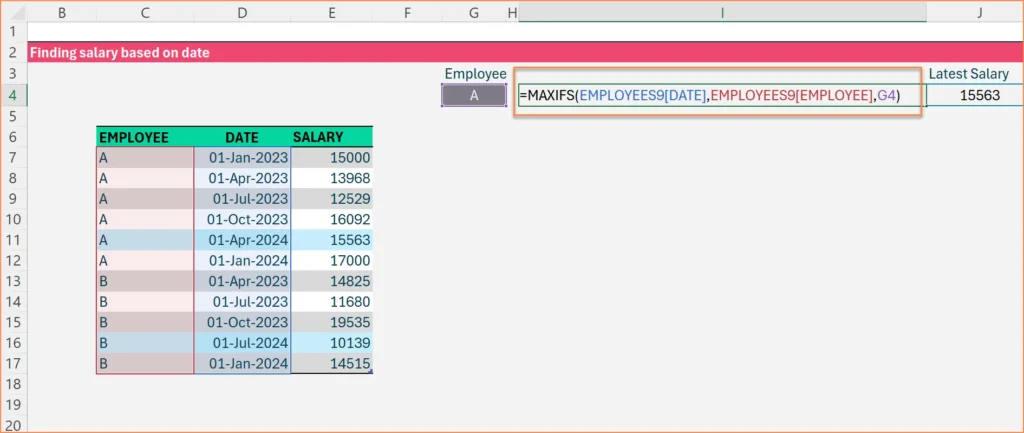
2. Now to get the salary of the employee on the max date, we will use the following formula.
=XLOOKUP(1,(EMPLOYEES9[EMPLOYEE]=G4)*(EMPLOYEES9[DATE]=I4),EMPLOYEES9[SALARY],"")Where cell I4 is the result of the MAXIFS done earlier.
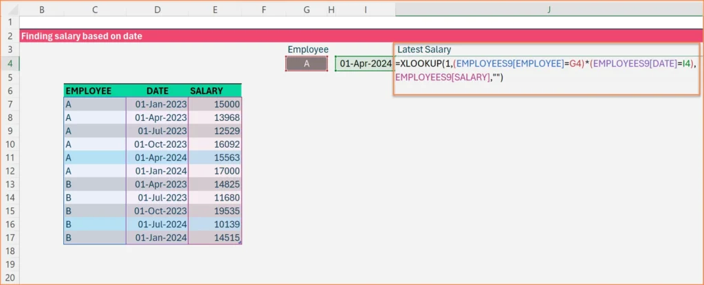
This will return the salary of the employee that equals the name of the employee in the cell and the date equals the max date in the cell.


