Create a Dynamic Monthly Calendar with a Single Formula in Excel

This blog addresses a more visually engaging task—creating a dynamic monthly calendar in Excel. By combining the SEQUENCE, DATE, and WEEKDAY functions, and by finding the first Sunday, creating a calendar is just a breeze with one single formula!

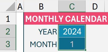
Consider, in our example, that the year and month inputs are in cells C2 and C3 respectively.

To generate a dynamic calendar with these inputs, we follow a 3-step approach:

1. Find the Sunday of the starting week.
2. Generate the sequence of dates.
3. Highlight only the current month’s dates using Conditional Formatting

Before we look into these steps, we recommend reading our blog on identifying the first Sunday of the first week of a month since we’ll use this in our steps here.

Now, let’s look at each of these steps in detail.

Step 1:

We will get the first Sunday of the month by using the DATE and WEEKDAY functions.  

The DATE function takes as arguments a year, month, and date and returns the corresponding date. The WEEKDAY function takes as input a date and returns its corresponding number.

In our example, year and month inputs are in cells C2 and C3, our formula would be:

= DATE($C$2,$C$3,1)  - (WEEKDAY(DATE($C$2,$C$3,1))-1)

For absolute cell references, lock the cells with the $ symbol as in the above example. This can be achieved by pressing F4 while writing the formula. 

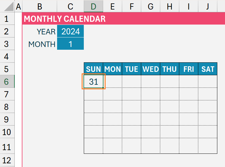
This gives us the first Sunday of Jan 2024 in cell D6:

Step 2:

With the first Sunday in hand, all we need to do is use the SEQUENCE function to generate a sequence of calendar dates.

In our example, we need a matrix of dates that resembles a calendar. For every month, there can be a maximum of 6 weeks (rows) and a week has 7 days (columns). The starting point will be the first Sunday from step 1 and increment 1 day as we need all the days.

With this, our formula will be:

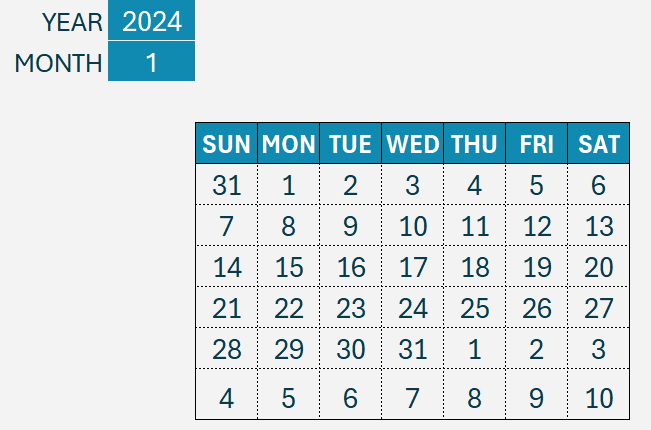
=SEQUENCE(6,7,DATE($C$2,$C$3,1)  - (WEEKDAY(DATE($C$2,$C$3,1))-1),1)

This generates the entire 6 weeks of the calendar as shown:

Step 3:

For our final step, let us make our calendar look aesthetically concise. That is, we will highlight only the dates in Jan 2024.

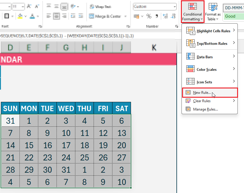
This is done by using conditional formatting:

1. Select all the cells, go to Conditional Formatting, and select a new rule for these cells.

2. Use a Formula as rule, where we use the MONTH function where the month of the cell (from D6 onwards) is not equal to the input month in cell C3.

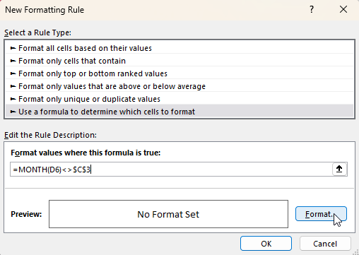
This formula applies conditional formatting only in the cells where the dates do not belong to the current month.

Note that while referring to cells in the formula, Excel automatically locks the reference with a $ symbol, edit the same wherever applicable. 

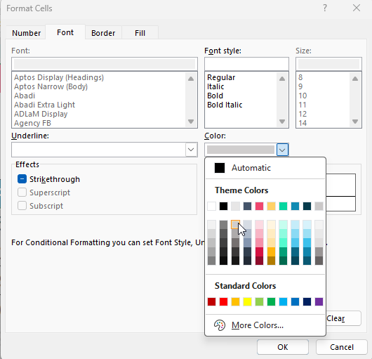
3. Now, we apply any format of choice to these cells and adjust the appearance according to our preference. Here, we’ve chosen them to appear less evidently than the dates of the current month by adjusting the fonts:

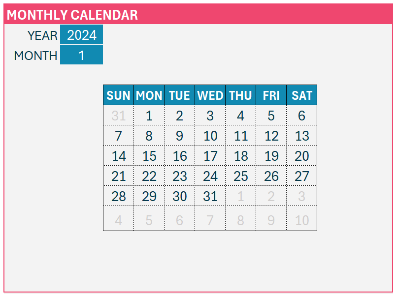
Now, our final, dynamic calendar will look like this:

Check our detailed, step-by-step video explaining the creation of this dynamic monthly calendar: