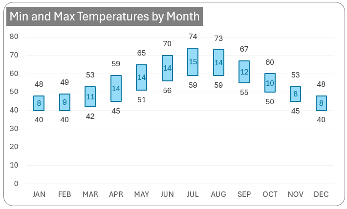
The Floating Column Chart (as shown below) is a powerful tool for showing ranges within your data. This type of chart is particularly useful for displaying minimum and maximum values, like temperature ranges or salary brackets, making it ideal for creating an impact in your presentations or reports.
With the amazing formatting options available in Microsoft Excel, building this chart takes just a few minutes. Let’s get started!
Ready to save time on your next presentation? Explore our Data Visualization Toolkit featuring multiple pre-designed charts, ready to use in Excel. Buy now, create charts instantly, and save time! Click here to visit the product page.
Do check our dedicated video on YouTube explaining these steps in detail.
The following are the steps we’d follow in creating this chart:
- Prepare the data
- Create a Stacked Column Chart
- Format to get a Floating Column Chart
- Add Min labels
- Add the Max series
- Modify the chart type
- Add Max labels
- Format for a visually appealing chart
Step 01: Prepare the data
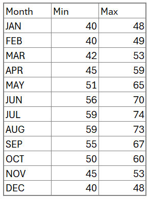
Consider sample data of minimum and maximum temperatures of a city for the year 2023.
For the floating column, we’ll create an additional column which is the difference between the maximum and minimum temperatures. Assuming our minimum temperature starts from cell C3 and maximum temperature in cell D3, our formula for this “Difference” column would be
=D3-C3With this, our sample data should look something like this:
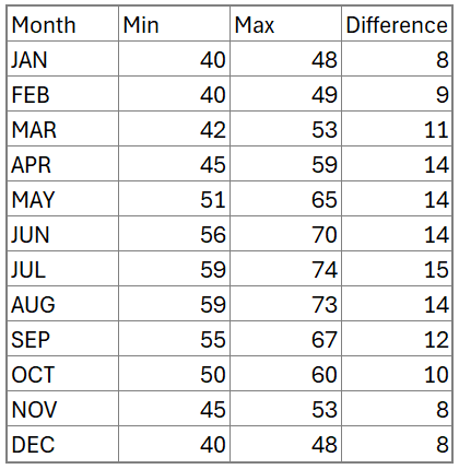
Drag the formula to populate the data in all necessary columns.
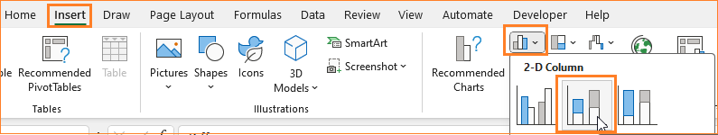
Step 02: Create a Stacked Column Chart
To create a chart, select the Month, Min, and Difference columns including the headers, and insert a stacked column chart.
Excel inserts a chart based on our data, as shown:
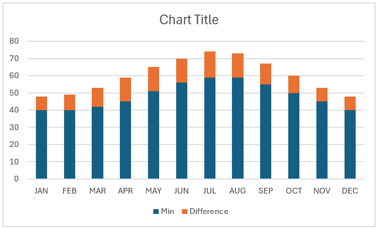
Step 03: Format to get a Floating Column Chart
To create a floating effect, we need to format the Min series. Right-click on any of the min column and go to format series to open the format pane.
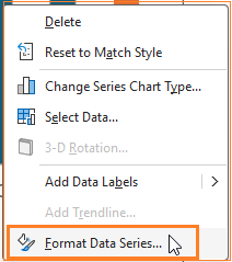
In the Fill & Line, remove the fill and border colors.
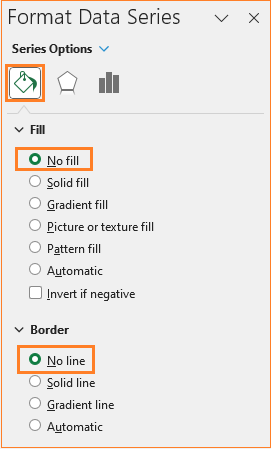
Similarly, right-click on the difference series and add data labels.
At this stage, our chart is:
In some cases, if the emphasis you are building is only on the difference between the min and max values, the above chart addresses the same and can be used as such.
Here, we aim to show the minimum and maximum values as well for that we need a few additional steps.
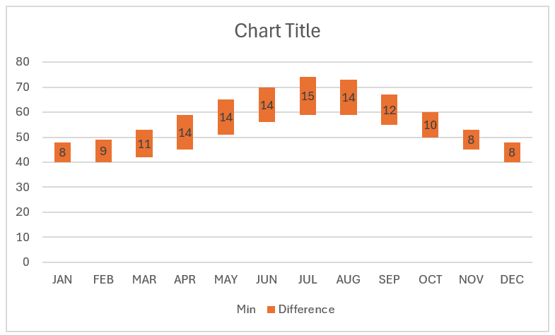
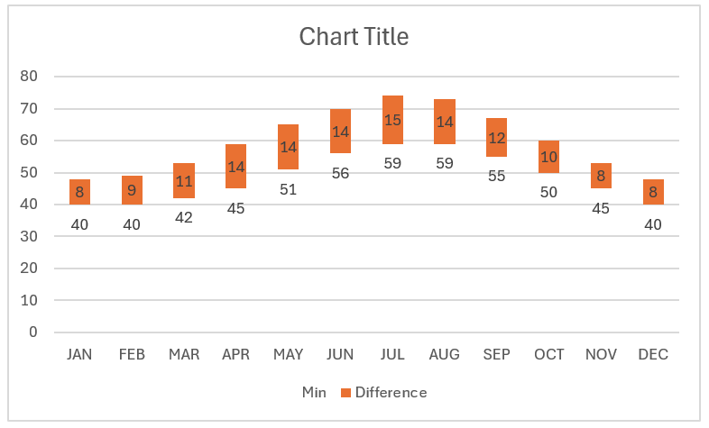
Step 04: Add Min labels
We already have a minimum series that was made “invisible” by removing the colors. To that, we’ll add data labels. Click on the min series, a “+” icon appears to the top right of the chart, from which choose to display the data labels:
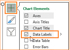
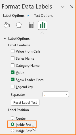
This inserts the labels, click on them and in the format pane adjust the position to inside end as shown:
By the end of this step, our chart looks something like this:
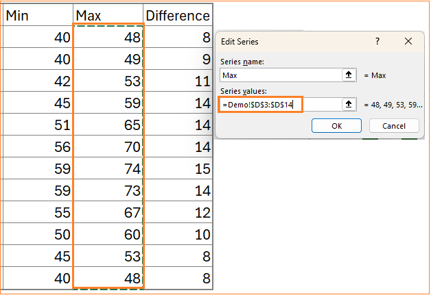
Step 05: Add the Max series
We can see that our chart is taking shape, we still need the maximum value labels to be displayed above the floating column.
To add this data, right-click on the chart and go to Select Data. This opens a dialog box, where we will add the maximum series.
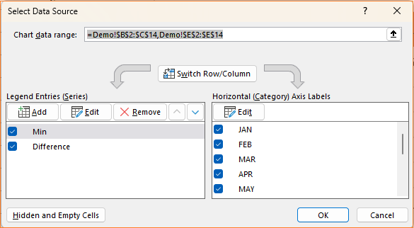
Add the max series as shown:
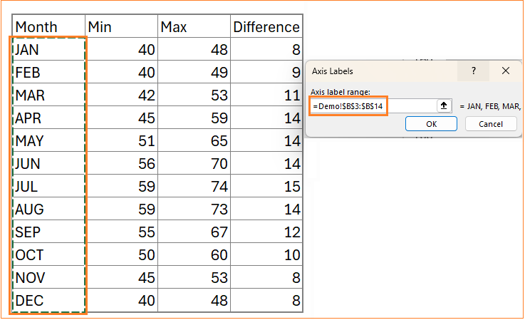
Add the Month column as the horizontal axis to this new series.
Adding this series modifies the chart as shown here,
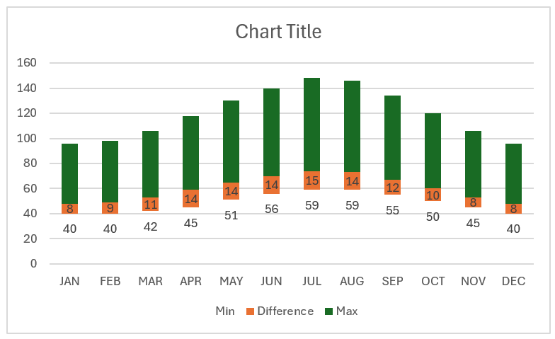
Let us format this to get the desired floating column chart.
Step 06: Modify the chart type
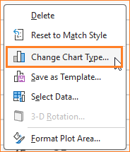
Right-click anywhere on the chart and go to Change chart Type which opens a dialog box.
In the dialog box, go to Combo and modify the Min and Difference series to be a Stacked Column chart and the Max to be a Line chart as shown here:
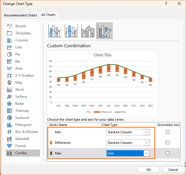
This again modifies the chart as shown in the preview from the above image.
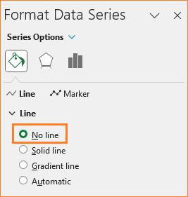
Step 07: Add Max labels
Click on the line and in the format pane, remove the line as shown:
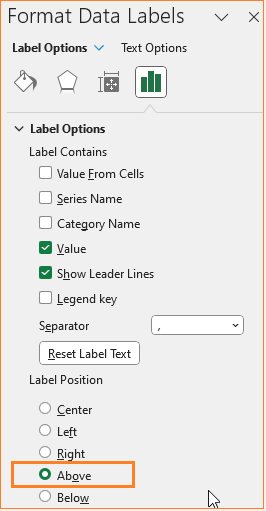
Now, in the “+” icon that appears on the top right of the chart, add data labels.
This adds labels, click on the labels, and in the format pane, adjust their position to “Above”.
With this step, our floating column chart is taking shape, as shown here. Now time for some final formatting to make this a visually effective chart.
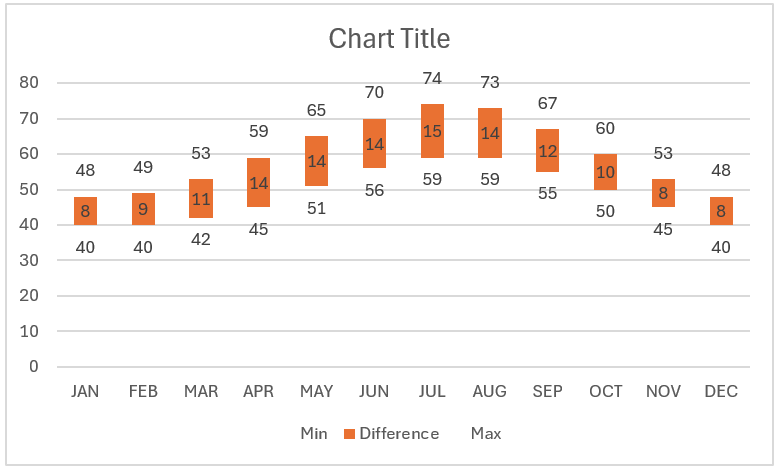
Step 08: Format for a visually appealing chart
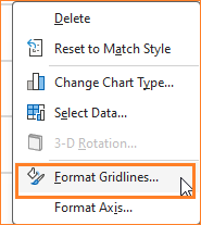
i. Now the gridlines, ensure to have them but not so evidently overpowering chart by modifying the line color.
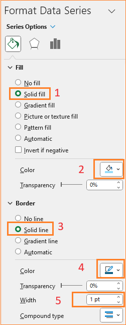
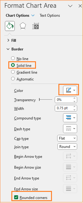
ii. To format the floating column, click on the columns and in the format pane, modify the color and the border color and width as shown here:
iii. Give a suitable title to the chart, say “Min and Max Temperatures by Month in 2023” and format the same in the Home ribbon.
iv. The legends here doesn’t add any meaning as our title is very clear on what the chart displays. Similarly, the axis titles here also not needed, so we’ll skip those.
v. As a final step of formatting, change the chart border by clicking on the chart and modifying the following in the format pane:
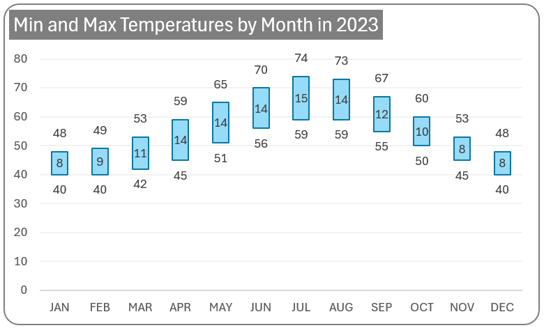
With this our floating column chart is ready!
Check our 1-page, downloadable illustrative guide explaining all the steps for a quick reference.

If you have any feedback or suggestions, please post them in the comments below.


