How to extend limits (tasks, time periods) in Gantt Chart Maker?
Our Gantt Chart Maker Excel Template allows creation of instant customized Gantt charts with a variety of options and features.
In order to keep the template file very light and fast, we establish some limits on the scope.
For example, the template handles up to 100 tasks, as the calculations are set up to handle only 100 tasks. The actual Gantt Chart display is designed in such a way that it fits in one page when printed. Hence it is limited in the number of time periods (52) and number of tasks (40) that are displayed.
In most common uses, 100 tasks should be sufficient. However, you may have to deal with a project with more than 100 tasks sometimes. Also, we may need to see more than 52 days at a time or more than 40 tasks at a time on the Gantt chart.
As all our templates are designed to be flexible, we can increase these limits with just a few quick steps.
EXTENDING THE LIMITS OF GANTT CHART MAKER
In this article, we will learn how we can extend the limits of the Gantt Chart Maker.
To demonstrate this, we will
- Increase tasks processed from 100 to 110
- Increase tasks displayed from 40 to 80
- Increase number of time periods from 52 to 104.
DEMO VIDEO
If you prefer video demos, please watch the video below where I walk through the steps. If you prefer screenshots and text, please continue further below.
OVERVIEW OF STEPS
- Extend number of tasks supported by template
- Extend the table in the hidden CALC sheet
- Extend number of periods shown on Gantt chart
- Unprotect sheet
- Unhide all columns.
- Copy column BL. Select extra 52 columns and Insert copied cells.
- Extend number of tasks shown on Gantt chart
- Copy Row 54. Select extra 40 rows and Insert copied cells.
- Change print settings to print the new expanded Gantt chart
STEP BY STEP INSTRUCTIONS
INCREASE NUMBER OF TASKS FROM 100
In this demonstration, I have entered about 110 tasks in the DATA_ENTRY sheet.
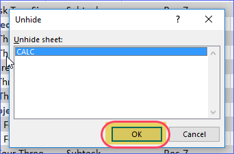
- First, unhide the hidden CALC sheet.
Right Click on the DATA_ENTRY sheet label and choose Unhide.
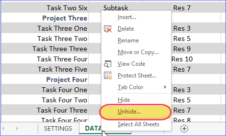
Select the CALC sheet and Click OK.
- Go to end of the calculation table
In the newly visible CALC sheet, go to cell AQ 102 (this is the end of the calculation table). One way to quickly get there is to press Ctrl+G. This opens the Go To dialog box as shown below.
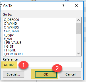
Type AQ102 in the Reference and click OK. This will move your cursor to AQ102 and make that as the active cell.
- Extend the formulas down
If you click on any cell outside the table, you can see that there is a small arrow at the bottom left of the cell AQ102.
Now, click on that arrow and drag the mouse down. This will now expand the table. The table that originally had 100 rows (from row 3 to row 102) will now expand as you keep dragging down.
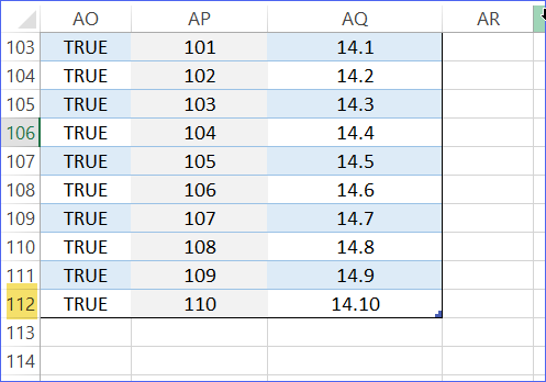
In this example, I am extending by 10 rows to row 112 and that will increase the number of tasks from 100 to 110.
You can increase to more tasks if needed. However, please keep in mind that the more we extend, more processing Excel has to do and can become slower gradually. So, extend only to as many tasks as you need.
- Hide the CALC sheet, as we don’t need it anymore.
Later in this article, we will prove that the template is now processing 110 tasks by displaying task #110 on the Gantt chart.
INCREASE NUMBER OF TIME PERIODS FROM 52 to 104
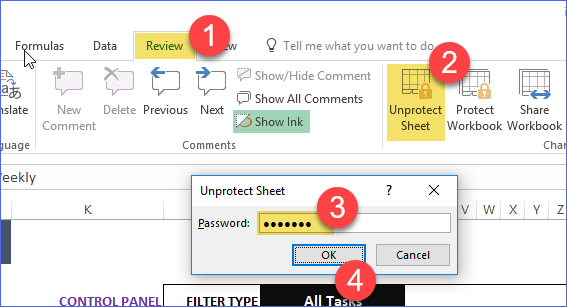
1. Go to the GANTT sheet and unprotect it.
Click on Review ribbon. Click on Unprotect sheet. Then, enter indzara as Password and click OK.
2. Now, we need to make room for the extra 52 columns.
Press Ctrl+A. This will select all cells in the sheet.
Now, in the HOME ribbon, in the Cells section, click on Format. Choose ‘Hide & Unhide’ and then select ‘Unhide Columns’
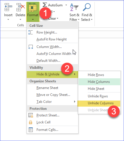
Now, you will see all the columns.
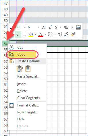
Right Click on column BL and click on Copy.
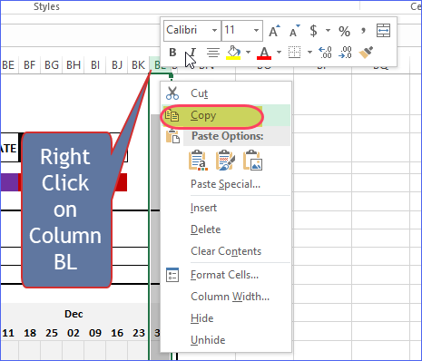
Select columns BM to DL and then right click to select ‘Insert Copied cells’
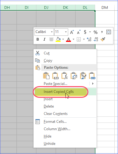
This will now insert 52 columns to our Gantt Chart display.
INCREASE NUMBER OF TASKS DISPLAYED FROM 40 to 80
1. Right click on row 54 label and choose ‘Copy’
2. Select rows 55 to 94 (40 rows) and right click to choose Insert Copied Cells.
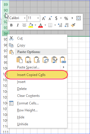
Now, the Gantt chart display has expanded to 40 new tasks, resulting in total 80 tasks.
If we enter 31 as the task that we want to begin with, then we will see tasks 31 to 110 (80 tasks displayed).
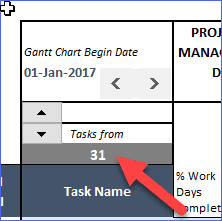
If you remember, we added support for up to 110 tasks earlier in this tutorial. Now, it is clear that the template is processing 110 tasks and can display 80 at a time on the Gantt Chart.
CHANGE PRINT SETTINGS
As we have expanded the width and the height of the Gantt chart, we have to change the print settings if you plan to print the entire Gantt chart. Originally, the Gantt chart printed on 1 page. Now, we will change to print on 4 pages, as we have doubled the height and the width of the Gantt chart.
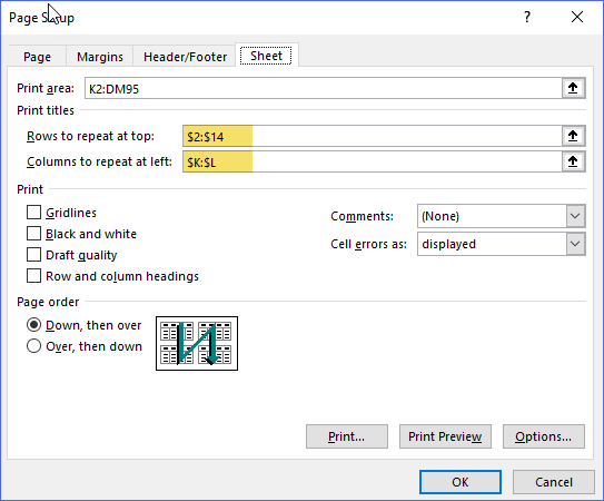
1. Click on Print Titles in the Page Layout ribbon.
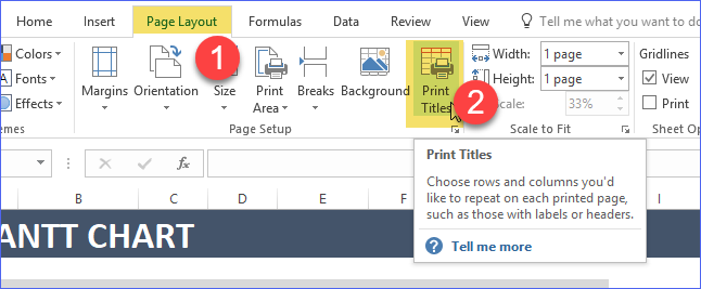
2. Select Rows 2 to 14 to repeat at Top. This will allow displaying the dates at the top in each page.
Select K and L columns to repeat at Left. This will allow displaying the Task name in each page.
3. Click on Page tab.
Select ‘Adjust to’ and enter 60% of Normal size.
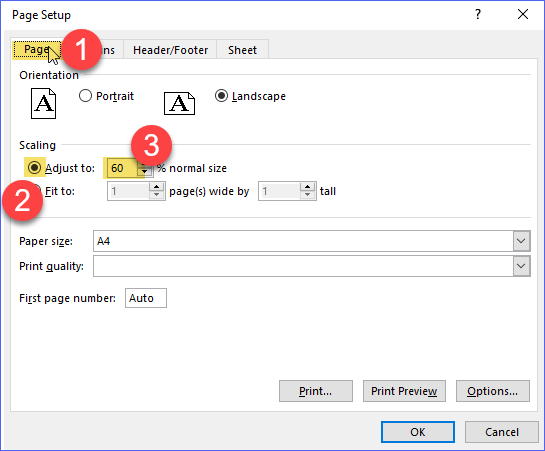
Click OK to close the window.
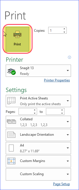
4. Now, press Ctrl+P to open the Print menu. The Gantt chart is now set up to print on 4 sheets.
Click on Print to print.
If you have any questions or suggestions, please post them in the Comments section below.
Leave a Reply