Calculating Average Employee Tenure in Excel

In this article, we will calculate a common HR KPI – Average Employee Tenure, using simple formulas in Excel.

Data

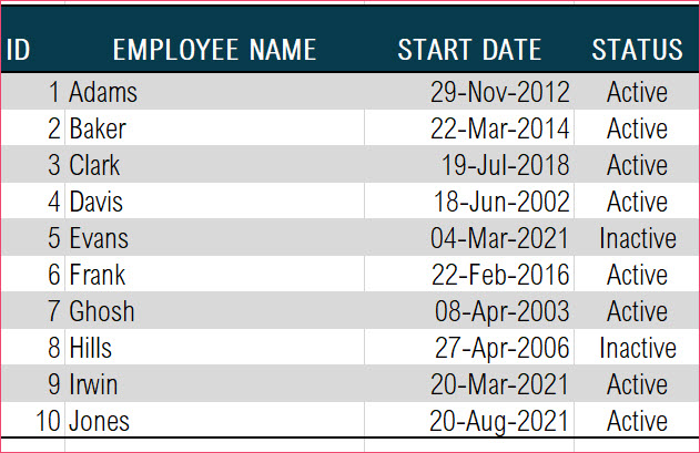
Let’s assume the dataset has a list of employees with a Status column to indicate Active vs Inactive employees. The table is converted to an Excel Table with name T_EMP

Definition

Tenure is the time from Employee’s Start date to Today. Average Employee Tenure is the average of all active employees in a company.

A longer average employee tenure indicates that employees are staying with the company for a long period of time which in turn means employees are happy and satisfied with the company.

Video Demo

Calculate tenure for each employee

Let’s first calculate tenure for each employee.

Since we want to do this calculation for each employee, we should store the today’s date value once and re-use, instead of calculating TODAY for each employee.  

Formula for calculating today’s date.

Formula

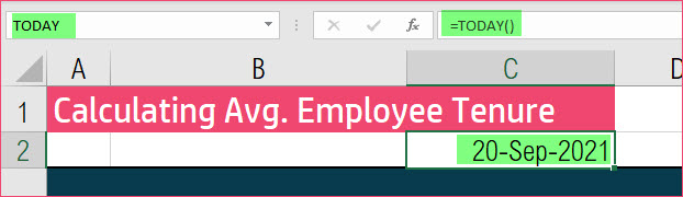
I am calling that calculated cell as TODAY (you can name it as you wish).

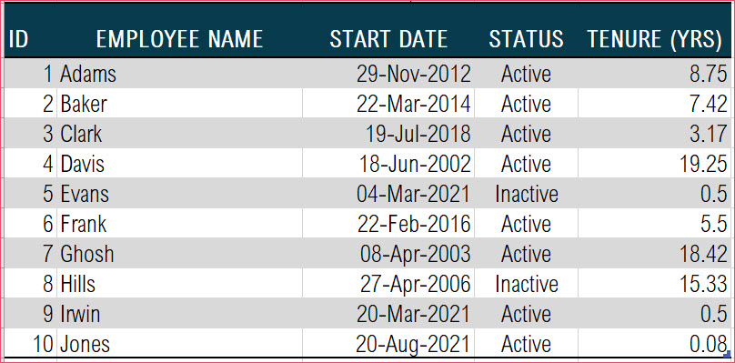
We can now write a formula for a new column ‘TENURE (YRS)’ in the table.

Formula

There are three operations we do in this formula

1. We use a function DATEDIF (which does not actually appear in newer versions of Excel – however if you type the function name and parameters, it works) to calculate the number of months from Start date to TODAY. The parameter “m” tells Excel to calculate the number of months.
2. I am first calculating the number of months and then divide by 12 to arrive at number of years including fractional year.
3. I then round to 1 digit using ROUND function to show tenure like “7.6 years”.

Now the table should look like below.

Now, let’s calculate the average tenure for all active employees.

Formula

There are two parts to this formula.

1. We use the AVERAGEIF function to only average the Tenure (Yrs) column if the Status is Active.
2. Then we round to 1 digit decimal place using ROUND function.

Bonus

As a bonus, to make the display show number of months, we could add another formula

Formula

G3 here represents the Average tenure in Years we calculated earlier.

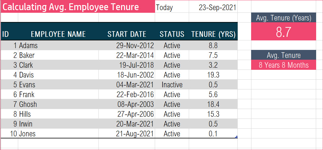
In the above example, we can see that the second display shows 8 Years 8 Months.

Functions used: DATEDIF, INT, ROUND, AVERAGEIF, TODAY

Conclusion

I hope this was useful. In your company, how do you calculate the average employee tenure? I would love to hear from you in the comments section.

Read More

• How to calculate number of Employees?