We’re focusing on comparing two lists to identify items that appear in either or both lists using conditional formatting. This comes particularly handy when you do not want to extract the values but to be able to visually see them in the original lists.
Being able to see items in a list in comparison with another list visually is useful in a lot of applications like:
1. Spotting unfulfilled orders by comparing lists of ordered versus shipped products.
2. In financial statements reconciliation compares lists of transactions from two different periods or sources.
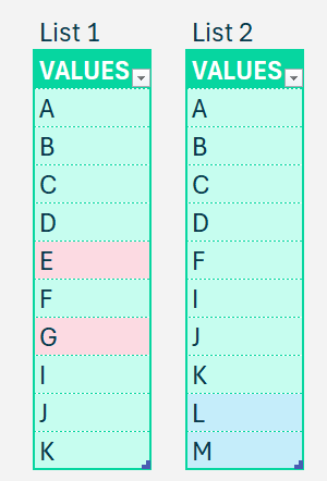
Consider two lists of items for a sample scenario.
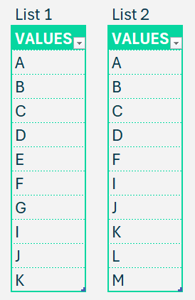
Before we get into the actual formulas for list comparison, let us get the data we have in the desired format:
First, convert these lists into Tables. LIST 1 is named TABLE1 and LIST2 as TABLE2
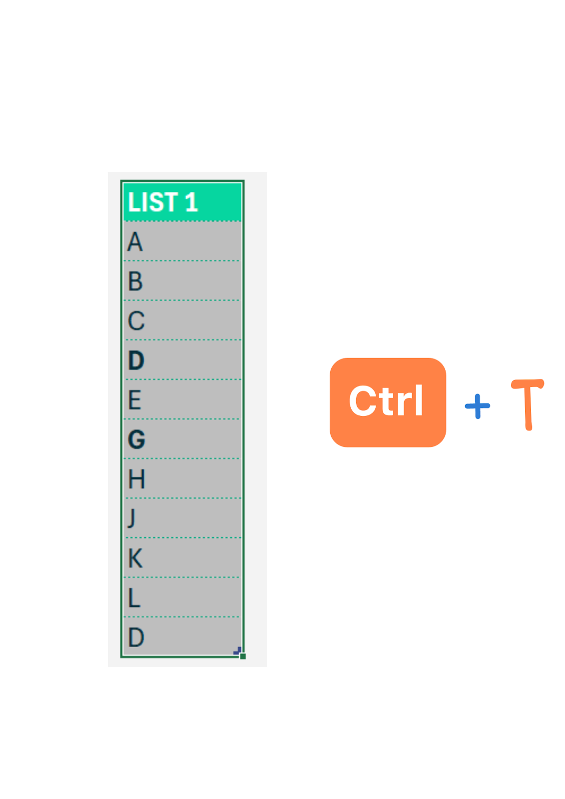
We create a table to increase formula readability and scalability when the data expands.
The second step is to create a List of the values in each table.
Though this is an optional step, we recommend doing this to ensure better readability of formulas. Achieve this by selecting all “values” in the table, go to the Formulas Tab and Define Name
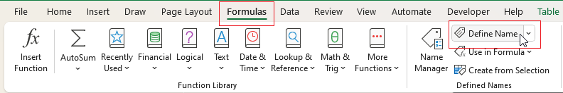
In our example, the first list is named List1, and the second is List2.
Now, let us get right into how to use conditional formatting to highlight items that are only in List 1 and those that are in both. The same logic will apply to the second list as well.
Let us understand the formula first and then use the same within conditional formatting.
Step 1:
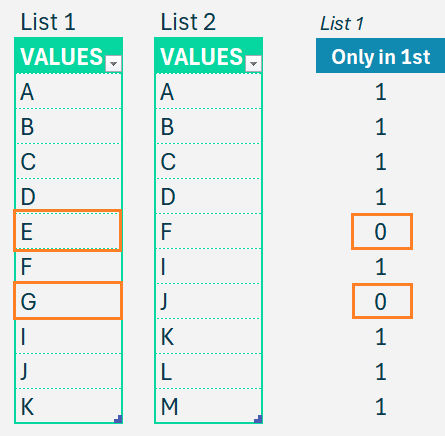
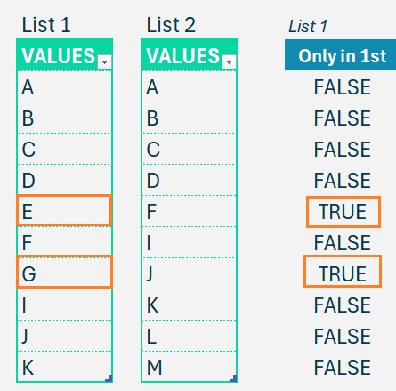
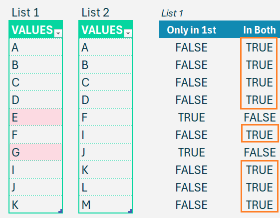
First, with a COUNTIF function to count within List2, the number of occurrences of every item in List1 (from cell C7 onwards). The formula goes like this:
=COUNTIF(List2,C7)For a better understanding, the COUNTIF function looks at the given range, searches for a given criterion, and returns the count of instances that meet the criteria.
The syntax for COUNTIF is

In our sample data, item A occurs only once in List2 so the COUNTIF returns 1, Since items E and G are not in List2 they are returned as 0.
Step 2:
Now, to change the numbers arrived using the COUNTIF function, and to get the desired result, we simply equal the formula to 0.
=COUNTIF(List2,C7)=0What does this formula give us? This returns a TRUE in places where the COUNTIF was 0. Essentially, the items that are only in List1 are returned TRUE.
We got the desired formula to get only values or items that are in List1.
Step 3:
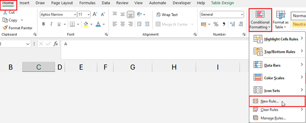
Now, apply conditional formatting on the original list. Select all the values in List1 and go to Conditional Formatting, New Rule in the Home Ribbon as shown.
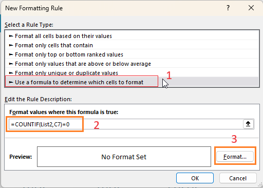
Select the Rule Type as “Use a formula …” and enter the COUNTIF formula we arrived at in Step 2.
Now all we need to do is apply the desired formatting for the cells where the formula is valid, do this by clicking on Format at the bottom of the window, as shown below.
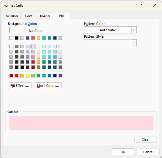
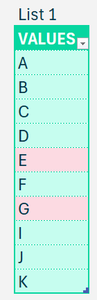
In this example, let us choose to “Fill” the unique item cells with Red. You can choose any formatting option you want.
Now once you click OK and apply all changes, you can visually see the list of items that are only in List1 highlighted on the list itself.

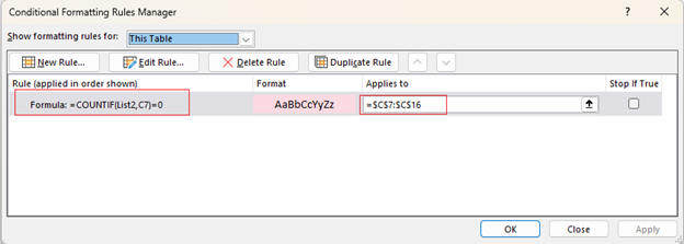
Always, while using conditional formatting, please ensure that your formula is correct and it is applied to your desired range.
To check, click on Conditional Formatting, then Manage Rule
Step 4
Now, let us proceed to highlight the list of items that are present in both lists. For this, copy the formula from Step 2 and instead of the COUNTIF equals zero, we choose values where COUNTIF is greater than zero.
=COUNTIF(List2,C7)>0Essentially, this formula returns TRUE to all items that are present at least once in List1 and List2.
Step 5:
All that we need to do now is to apply this formula as conditional formatting to our List1 (follow step 3) and choose a different color/format to highlight, as per your need.
Step 6:
Now that we know how to identify and highlight items in List1, the same logic can be applied to highlight items in the second list as well.
=COUNTIF(List1,E7)=0This counts the number of times the value in cell E7 appears in List1.
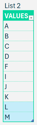
Step 7:
Similar to step 3, apply the formula as a conditional formatting. Here, in our example let us use blue to highlight these values.
Step 8:
To get the items that are in both lists, modify the previous formula similar to step 4. We need TRUE for items that appear at least once in both lists.
=COUNTIF(List1,E7)>0Apply similar conditional formatting as above, to highlight the items in both lists in green (you can choose formatting that best suits your needs).
That is all, the final lists are visually easy to read.
We have a dedicated video on comparing lists using conditional formatting, check it out:
If you are interested in extracting the items in a list using formulas, read our blog on comparing lists with formulas.
If you have any feedback or suggestions, please post them in the comments below.


