In Excel, there are multiple ways of comparing lists, this blog focuses on using Power Query for the same.
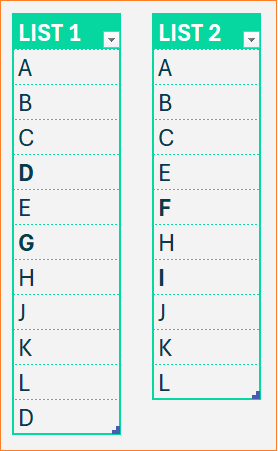
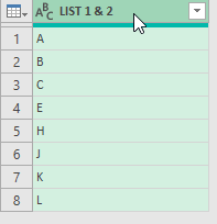
For a sample scenario, consider two lists of items as shown here:
Some use cases where such comparisons are useful: Consider you have lists of customers who purchased products A and B. Comparing these lists to get the list of customers interested in both your products or only one. This comes in handy to analyze and strategize your product development and marketing campaigns.
Check our detailed video on the steps to follow:
Please note that, these two lists are converted into tables called TABLE1 and TABLE2 before we begin our steps.
Step 01:
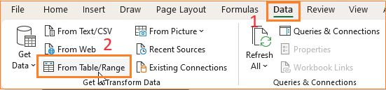
To begin, we need our data in Power Query. For this, click anywhere inside the table (say TABLE1) (1) Go to Data (2) Get Data from Table/Range:
This loads our TABLE1 into Power Query.
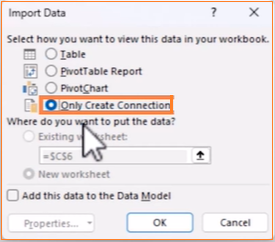
As our data is already in tabel format, there isn’t much to change here. So, we can close and load this back into Excel. This opens another pop-up to choose how we’d want this to load as? Since it’s a table already we’ll create only connection now as shown:
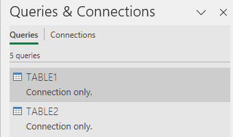
In this same manner, load the second table into Power Query.
Step 02:
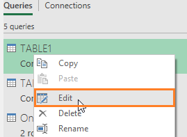
With our initial set-up done, click on Edit inside any connection to get back into Power Query.
Let us first identify the items that are ONLY in the first list.
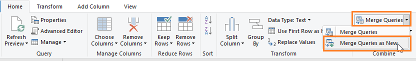
Click on the TABLE1 query (1) Go to Merge Queries (2) Merge Queries as new
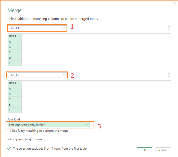
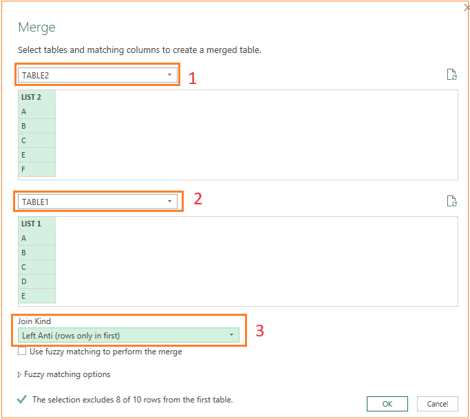
This opens another window where we can choose what and how to merge this data as.
We need this to be merged with TABLE2 where we need items only from TABLE1.
For this, choose the Left Anti (rows only in first) option, as shown here:
This results in the creation of a new query on the side panel, renamed as needed (OnlyinList1).
We’ll do some cleanup in our data. We can remove the TABLE2 from this.
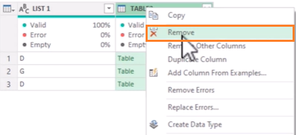
We’ll also remove duplicates as we can observe that there are two items “D”s in the list.
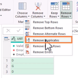
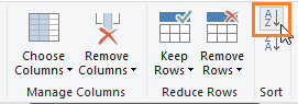
As a final step, let us sort our data in ascending:
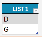
This will give us the list of items only in the first list. Which we’ll load back into Excel.
For this, click on “Close & Load” and “Close and Load to..”
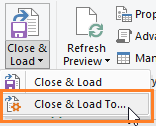
an existing location in the sheet per your need as shown:
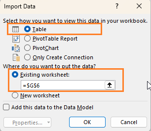
We can apply formatting as needed and have the items that are only in TABLE1 as shown:
Step 03:
To extract the items that are only in TABLE2, we’ll repeat the process from step 02 with just one change when we create a new merge query.
Click on TABLE2 and merge queries as new with the TABLE1 as shown:
This creates a new query, let’s name it OnlyInList2.
Repeat the same process of removing TABLE1, removing duplicates, and sorting.
Note: Even in the absence of duplicates, perform the same steps to ensure that when new data is added, Power Query can perform all these steps with just a single refresh.
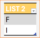
Close & Load into an existing location in the same sheet. This creates our new table with items only in TABLE2.
Step 04:
Let’s learn how to extract items from both the lists.
Follow the same initial steps, click on TABLE1, and Edit to open Power Query, in the Merge Queries as New, apply the “INNER JOIN” which extracts items from both lists.
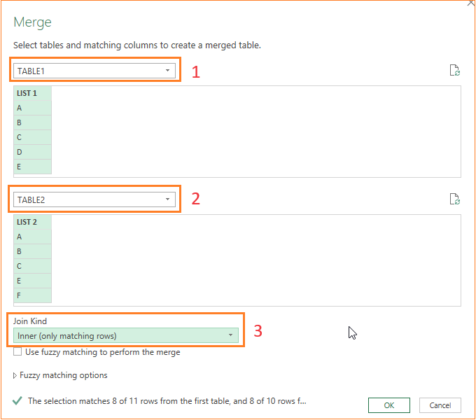
Repeat the same steps and rename the query (InBothLists) and the column name as shown here:
Now, remove duplicates and sort; close and load to an existing location.
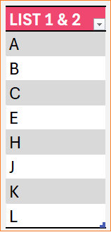
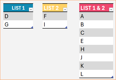
After some formatting to the table, we’ll have our final list of items from both tables:
With this, we have compared and extracted the items in one or both tables using Power Query.
To check the dynamic nature of this, add/modify data to the original tables and click in Refresh (Under the Data ribbon) to see the newly created tables update automatically.
Learn to compare lists using other methods in our blogs: using formuals, using conditional formatting.
If you have any feedback or suggestions, please post them in the comments below.


