Filtering data is a crucial part of data analysis in Excel, especially when dealing with large datasets. Excel provides various functions to filter data, and one such function is FILTER used in combination with SEARCH or FIND for text matching.
Scenario: Locating Employees Based on User-Input City
Consider an HR department that needs to quickly locate all employees based in a city specified by the user. Perhaps there’s an upcoming regional meeting or a need to assess the number of employees in a particular location for a new office setup.
There is an existing data set (as a table EMP_DATA) in Excel where all the details of the employees are stored.
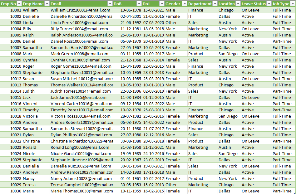
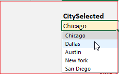
In our dataset, let’s assume users will input their desired city into a named range called CitySelected.
We want to filter the dataset to extract all employees whose location contains the city name provided by the user. Along with this we need only select information from the employee table like the ID, name, email address, and the department.
Note that these are not adjacent columns in the given data.
The FILTER Function
The FILTER function in Excel, which has the following syntax:

Our need here is to extract the number, name, email address, and department from the EMP_DATA table (the range) and the condition for filtering (criteria) would be that the CitySelected is equal to the Location column data from the employee table.
First, the EMP_DATA table DOES NOT have all of these ranges as adjacent columns so our range to filter needs to be extracted using an INDEX function. This will be:
=INDEX(EMP_DATA,SEQUENCE(ROWS(EMP_DATA)),{1,2,3,7})The syntax for the Index is:

What’s happening here?
We have used the INDEX function to retrieve all the rows of data from the EMP_DATA table (the SEQUENCE function takes care of this) where the columns are only what is required as specified within the curly braces (columns 1,2,3,& 7).
We have the range to filter. The criteria the filter function needs to satisfy is the CitySelected is equal to the Location column data from the employee table.
This is achieved using the SEARCH function:

In our case, this part of the formula will be:
SEARCH(CitySelected, EMP_DATA[Location])
Please note, that for case-sensitive searches, use the FIND function in place of the SEARCH function.
This will return a number for every successful match and return an error when there is no match. We’ll wrap our SEARCH result with an ISERROR function to return 0 in case of an error:
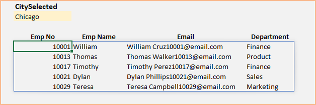
Over this, our filter condition is only when we get a match ie. for values >0. With this, our final formula will be:
=FILTER(INDEX(EMP_DATA,SEQUENCE(ROWS(EMP_DATA)),{1,2,3,7}),(IFERROR(SEARCH(CitySelected,EMP_DATA[Location]),0)>0))The employee data with the filter based on location will look like:
This method allows HR managers to dynamically search and filter the employee database based on specific text input, such as a city name.
It’s an efficient way to handle queries that require quick access to subsets of data based on variable criteria.
This formula is used in one of our videos on creating an interactive NFL Team schedule:
If you have any feedback or suggestions, please post them in the comments below.


