In this post, let us look at how better we can visually present a data table with multiple columns: by sorting them.
Sorting your data based on multiple columns is useful in a lot of real-life scenarios like:
Working with sales data, you should sort by date and then by sales amount to see the progress of sales over time and much more!
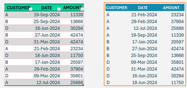
Consider, a sample data of customers with date of payment and amount,
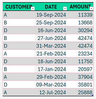
We shall look at how to sort this sample data by customer and then by date and amount.
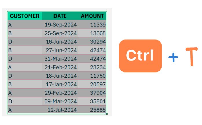
If you’ve been following our posts, one thing we always recommend is to convert your sample data into a table to ensure data readability and scalability when data expands.
To do this, select all data, press CTRL+T, and assign a name (say DATA).
Before we begin sorting our data with formulas, Excel has built-in SORT available. Go to the Data tab and click on Sort.
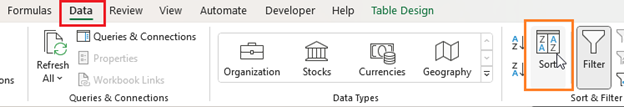
A pop-up window will appear and you can choose the column(s) and the order to sort.
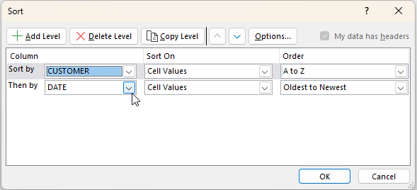
However, this is not dynamic. If you add more data to your existing table of data, you might want to do this Sort all over again.
Let us see how to use Excel formulas to sort data with multiple columns. To do this we will use the SORTBY function.
This function sorts or arranges data from a given range/array (1st argument) based on another range/array (2nd argument). You can also specify the sort order(3rd optional argument), that is either ascending (1) or descending (-1). You can add additional columns to sort by as the next arguments (optional).
To get a clearer picture, the syntax of SORTBY function is,

So, for our sample data, we shall sort the entire DATA table, first based on the CUSTOMER column in ascending order and, secondly by the DATE column in ascending order (chronological).
Our SORTBY for the sample data would be:
=SORTBY(DATA,DATA[CUSTOMER],1,DATA[DATE],1)And our sorted data would be
Apply conditional formatting
Since we are talking about data presentation in our article, let us highlight our sorted data, and to do this, we shall use conditional formatting.
There are numerous ways to highlight a dataset, in this case, we shall highlight every row that has a new customer.
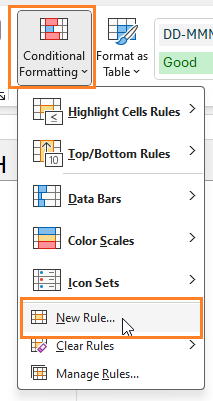
To achieve this, select all the newly sorted data, click on conditional formatting, and select a new rule:
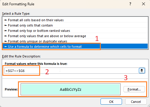
Since our data starts from cell G7, our formula should check the previous cell’s entry and if they are not the same, highlight it since it’s a new customer. The formula would be
=$G7<>$G6We’ll choose to format the cells in green.
So, the whole conditional formatting rule would be:
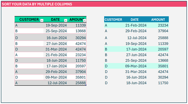
Once we apply this, our new sorted data will look like this:
We have a detailed explainer video on sorting multiple columns in Excel:


