The focus of this blog post from our “Data to Decisions’ series is on comparing two lists to identify items that appear in either or both lists. This is a common scenario when cleaning data for further transformations and analysis.
Why do we need to compare lists?
Consider you have lists of customers who purchased products A and B. Comparing these lists to get the list of customers interested in both your products.
This comes in handy to analyze and strategize your product development and marketing campaigns.
Another example would be in the reconciliation of financial statements. Here, identifying the list of transactions from only one system or those from both systems is a very common use case.
Let us learn how to do this with an example:
Consider two lists of items, LIST 1 and LIST 2.
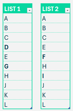
Before we get into the actual formulas for list comparison, let us get the data we have in the desired format:
First, convert these lists into Tables. LIST 1 is named TABLE1 and LIST2 as TABLE2
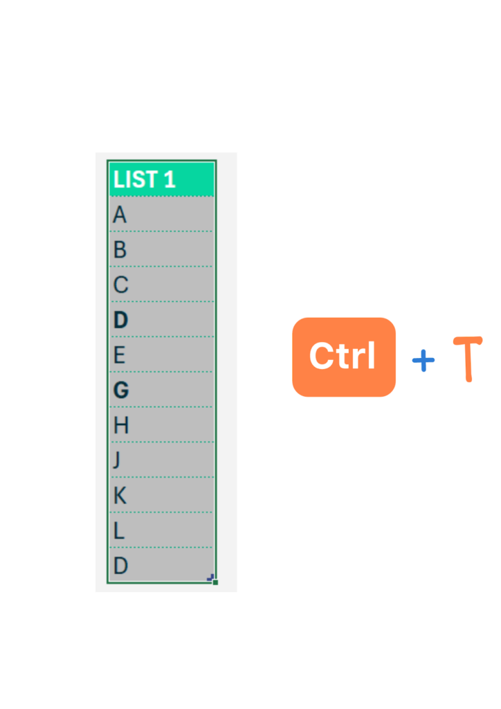
We create a table to increase formula readability and scalability when the data expands.
The second step is to create a List of the values in each table.
Though this is an optional step, we recommend doing this to ensure better readability of formulas. Achieve this by selecting all “values” in the table, go to the Formulas Tab and Define Name

In our example, the first list is named LIST1, and the second as LIST2.
With the named lists, let us get right into our formula building:
Let us work on the formula to get the list of all items that are only in LIST 1. Once we know how to achieve this, the same logic will apply to getting the list of items only in LIST2.
Get the list of items only in List1
Firstly, use a MATCH function to find values in LIST1 that are EXACTLY appearing in LIST2.
=MATCH(LIST1,LIST2,0)To understand this, let us look at what the Match function in Excel does.
The MATCH function in Excel is used to find the position of a specified item in a range of cells.

In our example, the first value in LIST1 is A, the Match function searches (or looks up) this value in LIST2 and returns the first position where A is found in LIST2, in our case 1. This continues for the whole LIST1.

We can see that since item D in LIST1 is nowhere found in LIST2, it returns #N/A error. Similarly for the value G.
To resolve this and proceed to get the list of values only in LIST1, we use the ISNA function and wrap the Match function.
=ISNA(MATCH(LIST1,LIST2,0))What does ISNA do? Wherever it encounters the #N/A error, it returns a boolean value TRUE.
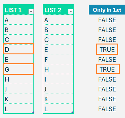
What does the above list tell us? The values returned as TRUE are only those in LIST1.
We are inching closer to our desired result!
Now, let us FILTER in the above formula to get only values that are TRUE from my original list.
=FILTER(LIST1,ISNA(MATCH(LIST1,LIST2,0)))The Filter function returns only those values in LIST1 that are TRUE based on its second argument (criteria).
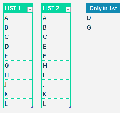
That is all! This gives us the list of items that are ONLY in LIST1.
Another important thing to remember while working with lists is that we might need to extract UNIQUE values in some cases. To achieve this, we wrap our formulas with the Excel UNIQUE function.
=UNIQUE(FILTER(LIST1,ISNA(MATCH(LIST1,LIST2,0))))Get the list of items only in List2
Applying a similar logic, we can get the list of items that are only in LIST2.
Here we match items in LIST2 with LIST1 and filter items from LIST2, so our formula would be:
=UNIQUE(FILTER(LIST2,ISNA(MATCH(LIST2,LIST1,0))))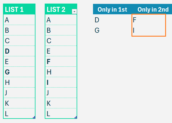
Get the list of items in both lists
This is quite simple while using the MATCH function (in Get the list of items only in List1), the values that are present in both lists return a NUMBER.
Now, instead of the ISNA function, we’ll use the ISNUMBER function to get items that match. So, the whole formula, to get the list of items in both lists is:
=UNIQUE(FILTER(LIST1,ISNUMBER(MATCH(LIST1,LIST2,0))))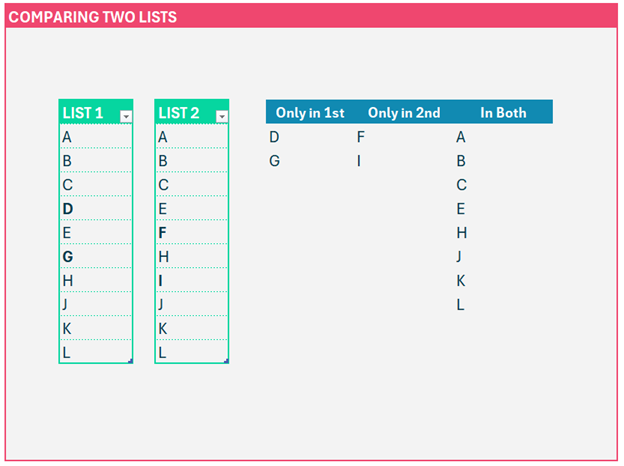
If you love a YouTube tutorial video, we’ve got you covered too!
We have a dedicated article on comparing two lists with conditional formatting.


