In this post from our “Data to Decisions” series, we focus on a common scenario Excel users encounter while working with lists: Extracting Top or Bottom N values from a list.
This technique is particularly useful in situations where you need to extract Top / Bottom customers by revenue, products by sales figures, students by their exam scores, and much, much more!
Read along to use powerful Excel formulas to achieve this dynamically!
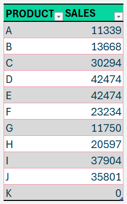
To begin, let us assume a sample dataset with a list of products and their corresponding sales as given below.
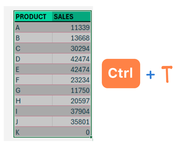
In most of our articles, we recommend using Excel tables, wherever possible to make working with formulas a lot easier. Let us create a table for our data and name it SALES.
Create a table by selecting the entire data, CTRL+T, and name your table as needed.
Let us dive right in to extract the Top/Bottom N values.
Step 1:
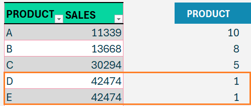
Here, we’ll use Excel’s RANK function to first rank the products based on the sales value.
=RANK(SALES[SALES],SALES[SALES],0)Let us understand the formula, by looking at what the RANK function does. The syntax is:
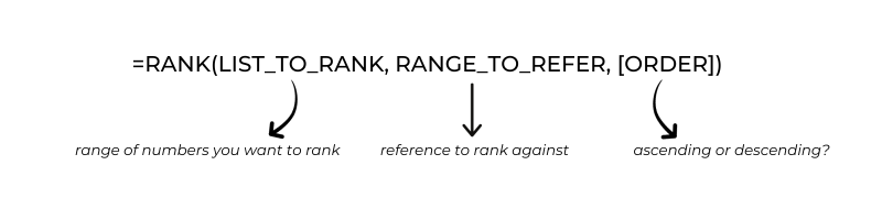
This function essentially returns a rank (as a number) to the list of values or items based on the range to refer in our case the products are ranked based on their sales. How to order this? We chose 0 for descending order as our third argument.
This gives us,
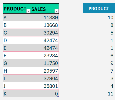
Note that here the Rank function assigns rank 1 to both products D and E since are of the same sale value.
Step 2:
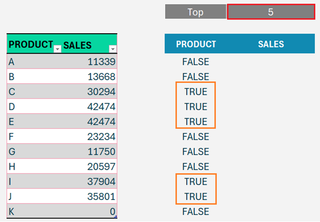
With the ranks of all products in hand, we’ll look at limiting it to a user-given value (in cell G4). To do this, apply the formula where the rank function is less than or equal to the N value in G4.

=RANK(SALES[SALES],SALES[SALES],0)<=G4This gives us TRUE for all the ranks that are less than or equal to 5 (as given by a user)
Step 3:
Proceeding to get the list of products and sales value based on a Top N or Bottom N given, let’s put to use the dynamic FILTER function.

The Filter function filters out an array based on a given condition and in our case, the condition is the Rank formula we arrived at in Step 2. That is the list of top N values from the table SALES.
So, our Filter function would be,
=FILTER(SALES,RANK(SALES[SALES],SALES[SALES],0)<=G4This returns the top 5 products and sales values. But the order of the sales value is not in descending order.
Step 4:
Hence, we’ll use the SORT function to sort based on the Sales column.
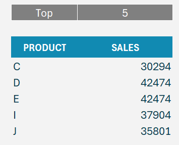
=SORT(FILTER(SALES,RANK(SALES[SALES],SALES[SALES],0)<=G4,2,-1)The syntax of the SORT function used here is
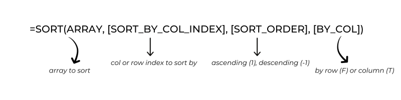
We are sorting the filtered list (as arrived in the previous step) based on the second column (the sales column) and the results to be displayed in descending order, hence -1. The result is:
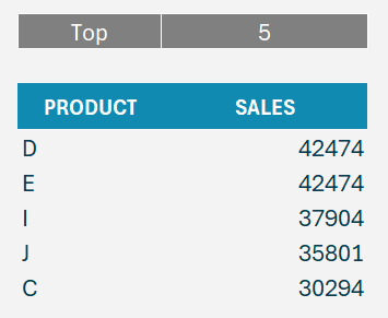
Changing the value in cell G4 changes the number of items in this list. Example,
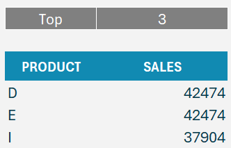
Please note that this function returns the exact count of N needed irrespective of the values being the same.
Step 5:
Let’s look at making this functionality dynamic. That is to be able to get either Top or bottom N values.
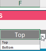
For our example, we have a simple drop-down created in cell F4 to choose either TOP or BOTTOM.
Step 6:
In the Rank function in step 1, we have included the third argument 0 to get the descending order, that is to get TOP values the rank needs 0 as the third argument, and 1 if it is BOTTOM values.
Hence, our modified, dynamic function for Top/Bottom values will be
=SORT(FILTER(SALES,RANK(SALES[SALES],SALES[SALES],

IF(F4="Bottom",1,0)

)<=G4),2, -1)
Step 7:
Now, similar to being able to select Top/Bottom, correspondingly the sort order for these values should be dynamic. To achieve this, the last argument of the SORT function needs to be modified.
That is, if the Bottom values are needed, the argument is 1 (ascending order) and if the Top values are needed, the argument is -1 (descending order).
=SORT(FILTER(SALES,RANK(SALES[SALES],SALES[SALES],

IF(F4="Bottom",1,0)

)<=G4),2,

IF(F4="Bottom",1,-1))
That is all you need to do to dynamically get TOP or BOTTOM N values from a list of values.
We have a detailed step-by-step tutorial on how to extract these values:


