This post from our “Data to Decisions” series is dedicated to calculating the profitability by product when you have a list of transactions (or orders) of the goods sold and the cost of each of these goods.
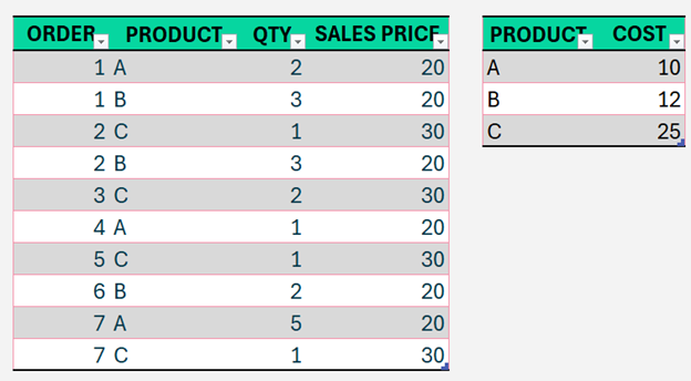
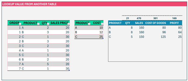
Consider a sample transaction list of products sold along with their quantity and sales price. Also, a product-level list of costs to produce the corresponding product.
For this sample, we’ll look at how to create a report that shows the profitability of each product. This report can be used to make key decisions like:
- Which products are more profitable?
- Identify those that are less profitable and take corrective decisions.
Before we begin, let us first convert our sample data into Tables. This is a step, we highly recommend to increase formula readability and scalability when data expands.
For this, select all the data, click CTRL+T, and assign a name to each table.
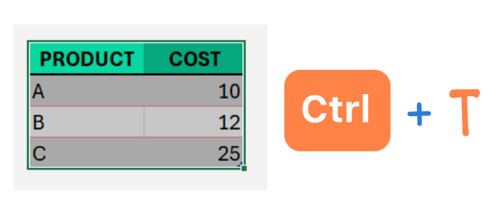
For the transaction details table, we’ve named it ORDERDETAILS and the product costs table as COST.
Let us get into a detailed step-by-step approach to generate the profitability by product report.
Step 1:
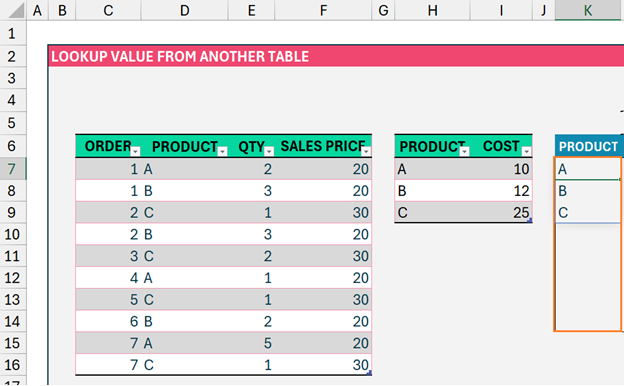
First, let us extract the distinct list of products from our ORDERDETAILS table by using the UNIQUE function. The formula in cell K7 will be:
=UNIQUE(ORDERDETAILS[PRODUCT])The UNIQUE function takes as input an array or range of data and returns only the unique list of values. Please read our blog on extracting unique values to know more.
Step 2:
Now, we will get the quantity sold for each product from the ORDERDETAILS table by using the SUMIF function, its syntax is as follows
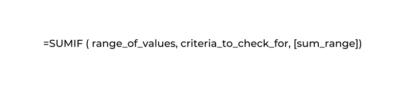
In our case, the formula in cell L7 will be:
=SUMIF(ORDERDETAILS[PRODUCT],K7,ORDERDETAILS[QTY])Note: Click and Drag the formula from cell L7 till wherever is needed to apply the same formula.
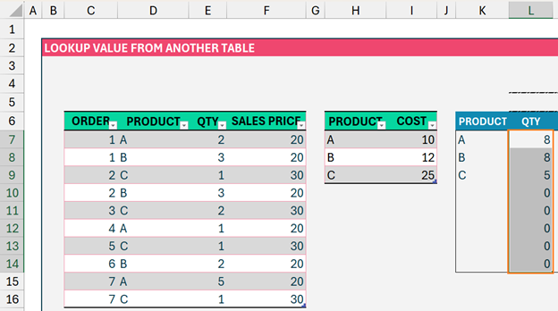
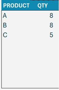
To remove the zeroes, we’ll enclose the above formula within an IF function, to display QTY only when there is a corresponding product. The modified formula will be,
=IF(K7="","",SUMIF(ORDERDETAILS[PRODUCT],K7,ORDERDETAILS[QTY]))The cleaned up, QTY details will look like this:
Step 3:
Let us now calculate the SALES amount. We’ll use the FILTER function over the ORDERDETAILS table to multiply the quantity and corresponding sales price but filter it based on the product in cell K7.
The syntax for FILER is,

Now our formula in cell M7 will be,
=FILTER(ORDERDETAILS[QTY]*ORDERDETAILS[SALES PRICE],ORDERDETAILS[PRODUCT]=K7This will return the sum of all product A sales based on the individual orders (orders 1,4 and 7). This looks like the below:
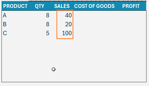
But, we need the sum of sales value for each of these products, so we’ll wrap the above formula with a SUM function. Similar to the previous step, we’ll also include an IF condition to return sales only when a corresponding product exists.
Our formula now will be:
=IF(K7="","",SUM(FILTER(ORDERDETAILS[QTY]*ORDERDETAILS[SALES PRICE],ORDERDETAILS[PRODUCT]=K7)))After Step 3, the report will look like this
Step 4:
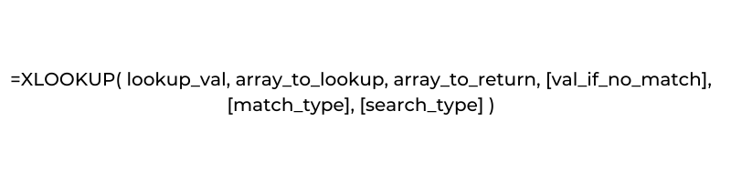
Here, we’ll calculate the Cost of Goods by using the XLOOKUP function. We’ll look up product A (in cell K7) from the COST table, and return the COST tables’ values.
In cell N7 our formula will be,
=XLOOKUP(K7,COST[PRODUCT],COST[COST]The syntax for XLOOKUP is:
The report will have the cost of product A in cell N7:
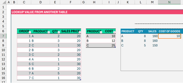
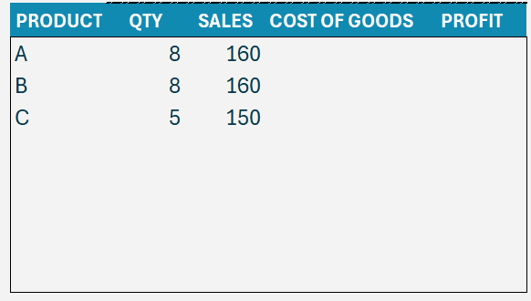
Since we need the total sales, we’ll multiply with the QTY of product A from our report (in cell L7). Similar to previous steps, we’ll wrap the whole function with an IF condition, our final formula will be:
=IF(K7="","",XLOOKUP(K7,COST[PRODUCT],COST[COST])*L7)The report will be,
Step 5:
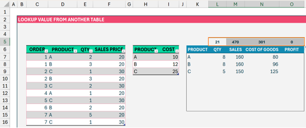
We’ll use the SUM function to calculate the total Quantity (in cell L5) as shown:
=SUM(L7:L14)Click and drag, horizontally to get the total Quantity, Sales, and Cost of Goods:
Step 6:
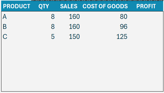
We’ll get into profit calculation now: this is straightforward, the sales value (in cell M7) minus the cost of goods (in cell N7) gives us the profit by product.
Here too, we’ll wrap this around an IF condition, our formula in cell O7 will be:
=IF(K7="","",M7-N7)Once this is calculated, our final report will have all the necessary details to make meaningful analyses:
We have a detailed, step-by-step explainer video on calculating profitability by product, do check it out:


