Excel’s FILTER function is a dynamic and flexible tool that can be used to display data based on multiple criteria. This function particularly is useful when dealing with a large dataset and only a handful of columns need to be extracted based on one or more conditions.
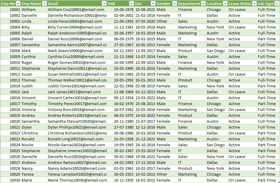
To see this function and its versatility in action. Let us consider a sample dataset of employee data of an organization as shown below.

This dataset (stored as a table structure named EMP_DATA) contains a lot of information about the employees. Say, for a report-building purpose, only select information needs to be extracted from this dataset. FILTER functions will be your go-to in such cases.
Let’s consider a sample scenario where based on a drop-down value of the Department name, we need to extract only the employee number, name, location, and job type.
Note that these are not adjacent columns in the given data.

The FILTER function in Excel, which has the following syntax:

Our need here is to extract the employee number, name, location, and job type from the EMP_DATA table (the range) and the condition for filtering (criteria) would be that the Department is equal to our input in cell C3.
The EMP_DATA table DOES NOT have all of these ranges as adjacent columns so our range to filter needs to be extracted using an INDEX function. This will be:
=INDEX(EMP_DATA,SEQUENCE(ROWS(EMP_DATA)),{1,2,7,10})The syntax for the Index is:

What’s happening here?
We have used the INDEX function to retrieve all the rows of data from the EMP_DATA table (the SEQUENCE function takes care of this) where the columns are only what is required as specified within the curly braces (columns 1,2,8,& 10).
We have the range to filter. The criteria the filter function needs to satisfy is the Department is equal to our input in cell C3.
That is, the final formula would be:
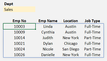
=FILTER(INDEX(EMP_DATA, SEQUENCE(ROWS(EMP_DATA)),{1,2,8,10}),EMP_DATA[Department]=C3)The fetched data will look like this:

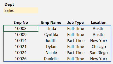
What if we need a different order of the above data, say Job Type comes before the Location of the employee?
The FILTER function can be modified to extract data in any order, our modified formula would be:
=FILTER(INDEX(EMP_DATA, SEQUENCE(ROWS(EMP_DATA)),{1,2,10,8}),EMP_DATA[Department]=C3)And our data:

The FILTER function in Excel is a potent tool to manage data efficiently. By combining it with other functions and features like drop-down lists and data validation, you can create interactive reports that update in real time based on your selected criteria.
This method of using filter function on non-adjacent columns of data is used in creating an NFL Standings visual, check the video on the same:
If you have any feedback or suggestions, please post them in the comments below.


